(1)
Department of Mathematics, University of Florida, Gainesville, FL, USA
11.1 Introduction
Zoonotic diseases are contagious diseases that are transmitted between animals and humans. These diseases are caused by bacteria, viruses, parasites, fungi, and prions that are carried by animals and insects.
Zoonotic diseases include vector-borne diseases but also diseases transmitted by vertebrate animals. For some zoonotic diseases, humans are a host that can pass on the pathogen to the animals or to the environment, while for others, the humans are a dead-end host. Examples of the first type are cholera, ebola, and malaria. Examples of the second kind are Rift Valley fever, hantavirus, West Nile virus, and avian influenza.
Zoonotic diseases play a very important role among human communicable diseases. In a review of more than 1400 pathogens known to infect humans, it was found that more than 61% were zoonotic [149]. Zoonotic diseases often serve as a starting point of many pathogens that jump the species barrier and become effectively human-to-human transmissible. Such diseases are called emergent diseases.
One of the most dangerous zoonotic pathogens is avian influenza H5N1. Avian influenza is transmitted from birds to humans. As of May 2014, H5N1 has infected more of 600 humans, 60% of whom have died. Besides the high mortality, what makes H5N1 dangerous is the possibility for the pathogen to mutate or reassort into a highly human-to-human transmissible flu pathogen with high mortality. In such a case, a world pandemic would occur, but since humans have no prior exposure to the H5 subtype of influenza A, mortality may be higher than it was in the 2009 H1N1 pandemic, caused by the “swine flu.”
11.2 Modeling Avian Influenza
Modeling zoonotic diseases in general, and avian influenza in particular, involves modeling transmission in several species. Many of the zoonotic diseases involve multiple species. For instance, the avian influenza pathogen infects wild birds, domestic birds, humans, and many animal species such as pigs and cats. One has to decide which species are important to the transmission.
In the case of avian influenza, we typically want to address questions related to human health. Humans are a dead-end host for H5N1, but H5N1 transmits to humans from domestic birds. It transmits effectively in birds and is endemic in the poultry populations in some countries.
11.2.1 Simple Bird–Human Avian Influenza Model
One of the simplest models of avian influenza (AI) was proposed by Iwami [80], following whom, we model transmission in poultry and the spillover to humans. H5N1 is very deadly for chickens. Mortality reaches 90–100% typically within 48 h [40]. This suggests that a simple SI model with disease-induced mortality is a good tool to model the transmission within poultry.

where S d is the number of susceptible birds, I d is the number of infected birds, Λ d is the recruitment rate, μ d is the poultry natural death rate, ν d is the disease-induced death rate, and β d is the transmission coefficient among poultry. Humans become infected from touching infected uncooked poultry products. The spillover model for humans takes the form

where S is the number of susceptible humans, I is the number of infected humans, Λ is the recruitment rate for humans, μ is the human natural death rate, ν is the disease-induced death rate for humans, and β is the transmission coefficient from infected poultry to humans.

(11.1)

(11.2)
The dynamics of the solutions to model (11.1)–(11.2) are not very different from those of the SI poultry model. The model has a reproduction number
 If
If  , then all solutions approach the disease-free equilibrium:
  . If
. If  , where
 We see that if β ≠ 0, then the outcome of the disease in humans is a direct consequence of the outcome of the disease in poultry.

 , then all solutions approach the disease-free equilibrium:
  . If
. If  , where
11.2.2 Parameterizing the Simple Avian Influenza Model
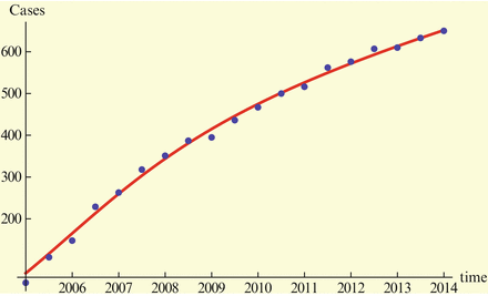
One of the main ingredients in developing models is determining reasonable parameter values for the model. We fix the time unit in years. The reason for that will become clear later. Determining parameters is typically done through fitting. Model (11.1)–(11.2) has eight parameters and four unknown initial conditions. The main data source is the cumulative number of H5N1 human cases given by the World Health Organization [166]. We give the data in Table 11.1.
Table 11.1
Number of cumulative human cases of H5N1 in units 105
Year | Time | Cases | Year | Time | Cases |
|---|---|---|---|---|---|
2005 | 0 | 0.00047 | 2010 | 5 | 0.00467 |
0.5 | 0.00108 | 5.5 | 0.005 | ||
2006 | 1 | 0.00148 | 2011 | 6 | 0.00516 |
1.5 | 0.00229 | 6.5 | 0.00562 | ||
2007 | 2 | 0.00263 | 2012 | 7 | 0.00576 |
2.5 | 0.00318 | 7.5 | 0.00607 | ||
2008 | 3 | 0.00351 | 2013 | 8 | 0.00610 |
3.5 | 0.00387 | 8.5 | 0.00633 | ||
2009 | 4 | 0.00395 | 2014 | 9 | 0.0065 |
4.5 | 0.00436 |
If the data are taken at half-year intervals, that will give 19 data points, potentially not enough to fit all parameters and initial conditions. A better approach is to predetermine some of the parameters. The Food and Agriculture Organization of the United Nations (FAO) publishes statistics on livestock [58]. FAO gives that in 2012, there were 24 billion units of poultry worldwide [58]. We set the world’s poultry population at 2400 × 107. Iwami [81] gives the mean lifespan of poultry to be two years. That translates into μ d = 0. 5. Since the entire population Λ d ∕μ d is equal to 2400 we have Λ d = 1200 in units of 107 per year. Iwami [81] also uses mean infectious period for domestic birds of 10 days, that is, ν d = 36. 5 years−1.
The natural lifespan of humans throughout the world varies significantly from country to country. We take an average value of human lifespan to be 65 years. Therefore, μ = 1∕65. The world human population has been on average approximately 6.5 billion over these 10 years. That gives a value of Λ = 1000 births per year in units of 105 individuals. Finally, we preestimate some of the initial conditions: S d (0) = 2400, I(0) = 0. 0007 and S(0) = 65000.
Alternatively, one can get the information about the poultry and the human population of only the affected countries, of which there are 16. Data exist in the same data sources. This is left as an exercise (see Problem 11.1).
To determine β d , β, I d (0), we fit the model (11.1)–(11.2) to the data, and we estimate I d (0) = 0. 3936, β = 0. 000000035327684, and β d = 0. 015489231377. The fit is given in Fig. 11.1. The Matlab code that executes the fitting is given in the appendix.
The estimated reproduction number with the fitted data is  .
.
 .
.11.2.3 Evaluating Avian Influenza Control Strategies
Control strategies that are currently in place have the goal of delaying or preventing the emergence of a pandemic H5N1 strain. These measures currently involve the following [108]:
Vaccination of poultry;
Culling/destroying infected and potentially exposed poultry;
Reducing contact with poultry by wearing protective gear;
Isolation of humans infected with H5N1 and tracing the source of infection of the isolated individuals;
Increasing biosecurity of poultry rearing;
Education of poultry workers and health personnel.
Multiple control measures are applied differently in different countries. Evaluating their overall effectiveness is not a trivial task. Typically, this is done by collecting the opinions of experts. Here we present a more objective approach. Suppose the goal of the control measures is to reduce the number of cases of H5N1 in humans, that is, the goal is to minimize I ∗. Each of the control measures impacts certain parameter values. We evaluate the change that a 1% change in a parameter p makes on I ∗ through the concept of elasticity. Recall that the elasticity of I ∗ with respect to the parameter p is given by

where
 We use Mathematica to compute the elasticities with the above-evaluated parameters. The elasticities are listed in Table 11.2.

(11.3)

Table 11.2
Table of elasticities of I ∗
Parameter | Elasticity | Parameter | Elasticity |
|---|---|---|---|
β d | 212.454 | β | 1 |
μ d | −215.338 | μ | − 1.00042 |
ν d | −210.569 | ν | − 0.999579 |
Λ d | 213.454 | Λ | 1 |
From this table, we see directly that control measures that are applied to poultry and affect poultry parameters are much more effective in influencing the prevalence in humans than control measures applied to humans. This result seems robust and independent of the model [108]. To compare the control measures, we determine which parameters each control measure would affect. For instance, culling affects μ d and ν d . Culling with repopulation affects μ d , ν d , and Λ d . Vaccination affects β d and ν d . Wearing protective gear affects β. We define the overall effect of the control measure to be the sum of efficacies of the effect of the measure on each affected parameter. For instance, culling with repopulation increases Λ d and increases μ d and ν d . Hence, the overall efficacy is 213. 454 − 210. 569 − 215. 338 = −212. 453. We will take this number as an absolute value. We summarize the overall effects of each control measure in Table 11.3. The affected parameters in the educational control measure are hard to pinpoint and are omitted.
Table 11.3
List of control measures and their efficacies
Control measure | Affected parameters | Overall efficacy | Rank |
|---|---|---|---|
Culling w/o repopulation | μ d , ν d | 425.907 | 1 |
Culling with repopulation | μ d ,ν d ,Λ d | 212.453 | 3 |
Vaccination | β d , ν d , β | 2.885 | 4 |
Biosecurity | β d | 212.454 | 2 |
Protective gear | β | 1 | 5 |
Isolation | ν | 0.999579 | 6 |
Table 11.3 suggests that culling without repopulation is the most effective strategy, but it is rarely applied. Without it, culling with repopulation and biosecurity are the two most efficient strategies, followed by vaccination. The low rank of vaccination comes from the fact that vaccination leads to asymptomatic diseases and increases the lifespan of infected poultry. At low levels, vaccination effectively supports higher prevalence. One caveat that we should mention is that the actual control measures do not necessarily affect all parameters with 1% change. Pinpointing the exact change is not trivial.
11.3 Seasonality in Avian Influenza Modeling
It has been known for a long time that human influenza exhibits seasonality in the temperate zones. In more tropical climates, human flu shows more complex patterns. The reasons for the human flu seasonality remain unknown.
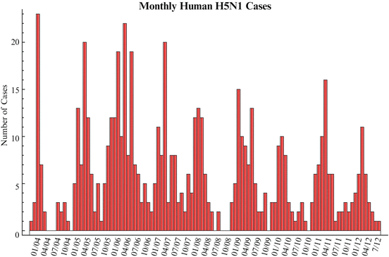
Avian influenza H5N1 affects many countries with different climates, and yet it exhibits seasonality similar to the human flu in temperate climates. This can be easily seen from the monthly human cases in Fig. 11.2.
Figure 11.2 shows that most of the cases occur in the period from December through March, and there are very few cases in the summer months. Moreover, in humans, seasonality can also be observed in H5N1 poultry outbreaks. To capture seasonality, we have to measure t in days or in months. Our preference will be to measure t in days.
11.3.1 An Avian Influenza Model with Seasonality
The cause of seasonality in H5N1 is completely unknown. Some authors have hypothesized that seasonality is intrinsic and should be modeled with autonomous models whose endemic equilibria can be destabilized and exhibit oscillations [107]. A more likely scenario is that seasonality is extrinsic. Perhaps the transmission rate β d is not a constant, but a periodic function of t, or the survivability of H5N1 in the environment is periodic. A recent study considered a number of potential extrinsic mechanisms and their combinations as possible drivers of seasonality in H5N1 [157]. The study performed model selection on the resulting seven models and found out that Iwami’s model with periodic transmission rate is the best fit to the cumulative number of human cases. We introduce that model here:

where the parameters have the same meanings as above. Seasonality is captured through a periodic transmission rate given by the periodic function

Here κ 1 is the amplitude, ω is the horizontal shift, and κ 2 is the vertical shift. We want κ 1 < κ 2, so that β d (t) > 0. The spillover model for humans takes the form


(11.4)

(11.5)

(11.6)
Model (11.4)–(11.6) is well justified. As before, it can be fitted to the cumulative number of human cases of H5N1. We show the fit in Fig. 11.3, where we fitted the data through December 2009. These data are called calibration data. Then we extended the solution and plotted it alongside the incoming new data, called test data. It can be seen that the model describes well the incoming new data.
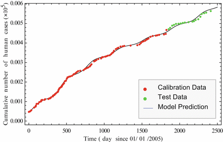

Fig. 11.3
Cumulative number of human cases of H5N1 in days
Model (11.4)–(11.6) is a model whose parameter β d is an explicit function of the independent variable t. We have not considered models of this type before. Recall, however, that models in which one or more parameters are given functions of the independent variable are called nonautonomous.
An important class of nonautonomous models consists of those in which the parameters are periodic functions of the independent variable.
Definition 11.1.
Models in which one or more parameters are periodic functions of the independent variable are called periodic or seasonally forced models.
Methods for nonautonomous models include the Poincaré map and Floquet theory. We direct the reader to the many excellent books that cover this topic [155].
11.3.2 Tools For Nonautonomous Models
There are many tools that are designed to facilitate the study of nonautonomous periodic dynamical systems. Nonautonomous periodic dynamical systems are to a large extent analogous to autonomous dynamical systems. Here we explore two such tools.
11.3.2.1 The Poincaré Map
The Poincaré map was developed to study the intersection of the solution flow of a periodic orbit with the transversal cross section S. It is a tool for investigation of the n-dimensional dynamical system


(11.7)
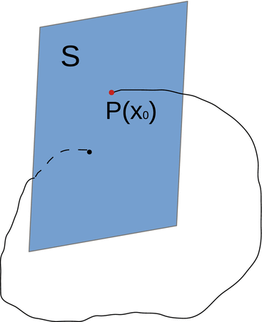
The Poincaré map is defined as the point of return of the periodic orbit to S.
Suppose the flow ϕ generated by (11.7) is T-periodic, that is, ϕ(t + T, x 0) = ϕ(t, x 0), and the cross section S of dimension n − 1 is transversal to the vector field. Then the Poincaré map  associates point x 0 in V with its point
  of the first return of the flow to S (see Fig. 11.4).
 associates point x 0 in V with its point
  of the first return of the flow to S (see Fig. 11.4).
