(1)
Multidimensional Microscopy and Cellular Diagnostics, Medical Faculty, Otto-von-Guericke-University, Magdeburg, Germany
(2)
Special Laboratory Electron- and Laserscanning Microscopy, Leibniz Institute for Neurobiology (LIN), Magdeburg, Germany
Abstract
Fluorescence lifetime imaging microscopy (FLIM) has become a powerful and widely used tool to monitor inter- and intramolecular dynamics of fluorophore-labeled proteins inside living cells.
Here, we present recent achievements in the construction of a positional sensitive wide-field single-photon counting detector system to measure fluorescence lifetimes in the time domain and demonstrate its usage in FRET applications.
The setup is based on a conventional fluorescence microscope equipped with synchronized short-pulse lasers that illuminate the entire field of view at minimal invasive intensities, thereby enabling long-term experiments of living cells. The system is capable to acquire single-photon counting images and measures directly the transfer rate of fast photophysical processes as, for instance, FRET, in which it can resolve complex fluorescence decay kinetics.
Key words
Time-correlated single-photon counting (TCSPC)Fluorescence lifetime imaging (FLIM)Förster resonance energy transfer (FRET)Positional sensitive photon multiplierMultichannel plate1 Introduction
1.1 High-Resolution Light Microscopy Beyond the Diffraction Limit
During the past two decades, the traditional fluorescence microscopy has developed from a discipline interested in the description of static microstructures to a tool of molecular cell biology aiming to analyze physiologically relevant molecular processes on the cellular and systems network level.
Exploring the dynamics and function of macromolecular networks requires high-resolution microscope techniques below the diffraction limit of visible light [1]. With the introduction of new microscopes and optical techniques, as, for instance, the introduction of multiphoton microscopy [2–5, 4pi-microscopy [6–10], stimulated-emission-depletion microscopy (STED) [11, 12], structured illumination (SIM) [13, 14], localization microscopy (ground-state-depletion microscopy (GSD)) [15], spatial precision-distance microscopy (SPDM) [16, 17], photoactivated localization microscopy (PALM/STORM) [18, 19], and light sheet illumination [20, 21], a significant improvement of spatial resolution beyond the diffraction limit of classical microscopy was recently achieved. Most of these concepts take advantage of the fact that fluorescence can be switched between a dark state and a bright state, either in a stochastic (PALM/STORM/GSD) or in a deterministic way (STED).
Unfortunately, most fluorescence microscopes work at high illumination intensities. The strive to collect as many photons as possible necessarily results in high average and peak powers [22] (typically >1 kW/cm2), which leads to irreversible photobleaching of dyes and significant photodamage of living cells [23]. Therefore, the abovementioned visualization techniques (1) do not allow the direct observation of molecular interactions over a longer period of time, (2) induce photodynamic reactions of the molecular probes, and (3) distort the living state. Prerequisite for non-distorted visualization of dynamic processes within living cells (e.g., during synapse formation and signal transduction) by fluorescence microscopy is a minimal invasive approach [24] to excite and detect the molecular constituents at conditions that preserve the undisturbed living state. Consequently, the development of minimal invasive observation systems that yield information about protein–protein or protein–target structure interactions on the cellular, subcellular, and single molecule level, without disturbing the intracellular metabolism, is an outstanding goal in modern cell microscopy.
1.2 Fluorescence Lifetime Imaging
The improvements of the spatial resolution in modern superresolution microscopes were an important step forward to visualize the molecular organization of cells but do not exploit the full informativeness of the fluorescence process. A fundamental technique capable to grant highest resolution, sensitivity, and comprehensive information about a fluorophore’s environment is fluorescence lifetime imaging microscopy (FLIM) (Fig. 1). Measuring the lifetime of the fluorophore’s excited state reveals incidents occurring in nanometer range of the molecular environment like changes in pH, temperature, ion concentration, viscosity, or polarity among others.
Fig. 1
Principle of FLIM. A basic single-photon counting setup comprises of a pulsed laser, a set of emission filters, a sensitive detector, and electronics for measuring time. The sample is excited with ultrashort laser pulses. Emission filters block the excitation wavelength of the laser and let the fluorescence pass. The detector generates an electrical pulse for each detected photon. This pulse is further electronically amplified and fed into a discriminator. The time difference between the moment of emitting the laser excitation pulse and the detection of the photon is measured
At present, two methods have been evolved to measure fluorescence lifetimes: frequency domain methods [25–27] and time domain-based methods [28–30] (Fig. 2a, b).
Fig. 2
Comparison between the principles of frequency-domain and time-domain FLIM measurement. (a) In frequency domain the fluorescence emission light (red line) is emitted with a phase shift ϕ after excitation by a modulated light source (green line). The amplitude of the emission light is characterized by the demodulation factor m. (b) In time-domain lifetime measurements, the sample is excited with a narrow pulse of light (green line). The emission intensity is detected (red line). The decay is well described by the exponential law and, therefore, looks like a straight line in log scale in case of a mono-exponential decay
Whereas in the frequency domain, the fluorescence lifetime is extracted from the phase shift and demodulation of the fluorescent light with respect to the phase and the modulation depth of a modulated excitation source, in time domain the decay information is acquired directly by recording the decrease of the fluorescent light intensity over time after exciting the specimen in a single-photon counting mode (Figs. 2b and 3). That means, a sample is illuminated with short laser pulses (fs to ps range), and the time difference between the emitted laser pulse and the appropriate fluorescent photon at the detector is measured resulting in a histogram of arrival times (Fig. 3). Among the other techniques, only single-photon counting is capable to utilize the detected photons as efficiently as it is physically possible [31] with short excitation pulses [32].
Fig. 3
Fluorescence decay acquisition using single-photon counting method. The sample is excited periodically with ultrashort pulses of light. The time difference δt i between the moment of the photon detection and the moment of the pulse emission is measured and stored for each registered photon. A histogram of the arrival times δt is build. The values of the histogram relate to the intensity integral inside the interval ΔT
1.3 Detectors for Measuring FLIM
A large number of detection techniques are employed for FLIM applications nowadays. The most widespread detectors, implementing single-photon counting-based approach, are photomultiplier tubes (PMTs) (Fig. 4, see Note 1), microchannel plate-based PMTs (MCP-PMTs) (Fig. 5a, c, see Notes 2 and 3), and single-photon avalanche diodes (SPADs) (see Note 4). In addition there are a number of integrating (opposite to counting) detectors: gated CCD cameras (Fig. 6, see Note 5), streak cameras (see Note 6), and conventional photodiodes. Advantages and drawbacks of the individual systems are listed in Table 1.
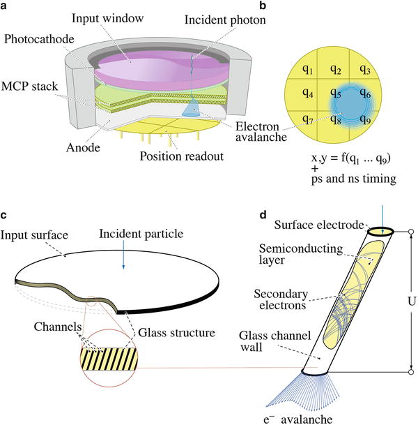
Fig. 4
Principle of a conventional photomultiplier tube (PMT). An incident photon strikes the surface of a photocathode and releases a photoelectron, which follows an applied electrical field towards a dynode system thorough the focusing electrode. Dynodes have a voltage gradient to accelerate secondary electrons and deliver more and more electrons. The anode electrode acquires all the electrons, resulting in a sharp current pulse
Fig. 5
Detector head. (a) Scheme of the microchannel plate (MCP)-based photomultiplier tube. The photocathode converts an incident photon to a photoelectron. A stack of two MCPs multiplies the photoelectron, and the resulting electron avalanche (indicated by a boxed area in a, b) is collected by a position-sensitive planar anode (b), which consists in the depicted case of a 3 × 3 readout pattern. (c) A microchannel plate is a glass plate of diameter varying in range of 18–80 mm that holds millions of individual channels 3–12 μm diameter. Input and output surfaces of a MPC are covered by a thin layer of metal for applying a voltage to grand electron multiplication. (d) Each individual channel of the plate acts like a miniature electron amplifier, because the inner walls of the channels are covered with a semiconducting layer (showing good secondary emission coefficient)
Fig. 6
Measurement principle of gated CCD. (a) A gated camera is a combination of a MCP-based light typically intensifier coupled to a CCD sensor by a fiber-optic window with a layer of phosphor as scintillator for back conversion of the electrons into photons. If the diameter of the intensifier is larger than the CCD-sensitive area, a fiber light guide is required to project the image to the sensor. (b) The fluorescence decay curve profile is acquired in several time windows (“gates”) along the time axis. (c) An interval of time within the photons are registered is formed by applying a voltage pulse in the photocathode–MCP gap. The duration γ and offset δt of the pulse define the period of the photons acquisition
Table 1
Advantages and disadvantages of various photon counting methods used for FLIM
Method | Advantage | Disadvantage |
|---|---|---|
Scanning FLIM | • High signal-to-noise ratio due to sensitive point detectors (SPADs) | • Count rate must be kept below excitation rate |
• Optical sectioning | • Accumulation of TCSPC signals necessary | |
• Lifetimes in combination with spectral detection | • Sequential data acquisition | |
Gated CCD | • Simultaneous lifetime information in whole image | • Loss of sensitivity due to discarding of photons |
• High-speed acquisition | • Limited lifetime accuracy | |
• High speed at cost of higher excitation power | ||
Wide-field FLIM | • Acquisition of all parameters describing the physical properties of individual photons | • Limited count rate |
• Minimal invasive excitation allows long-term observation | • Accumulation of photons |
1.4 Time and Position-Resolved Single-Photon Counting
In contrast to time only single-photon counting techniques that acquire positional information by scanning methods in a wide-field FLIM-system, a vacuum-sealed microchannel plate-based photomultiplier tube (MCP-PMT) with a positional sensitive multi-anode is used as detector.
A position-sensitive photomultiplier (see Note 3) combines a photocathode (see Note 7), a microchannel plate (MCP) stack (see Notes 2 and 3), and a position-sensitive anode system (see Note 8) (Fig. 5).
To register single photons, the detector needs an amplification element to convert single quanta of light into an electrical signal that can be processed and measured. This conversion process is performed by the photocathode. The photoelectron following an applied electrical field is subsequently multiplied by a microchannel plate stack (Fig. 5c). The resulting avalanche, depending on the number of amplifying elements, consists of 105 to 107 electrons. The avalanche is detected by an anode (Fig. 5a). A conventional disk or cone-like anode enables only time-resolved registration. Alternatively, the electron cloud is converted back to the visible light by a phosphor screen for CCD-based acquisition (e.g., gated CCD).
However, the latter approach cannot be used in applications where single particle counting is required because of the long readout time of a CCD. Therefore, it is necessary to employ a position-sensitive anode that provides spatial information for each individual detected event in combination with timing information.
2 Materials
2.1 Cell Culture and Transfection Reagents
1.
DMEM → Dulbecco’s Modified Eagle Medium.
2.
DMEM(+) → DMEM, 10 % fetal calf serum (FCS), 2 mM l-glutamine, 100 U/mL penicillin, 100 μg/mL streptomycin.
3.
Lipofectamine™ 2000 Transfection Reagent.
4.
PolyFect Transfection Reagent.
5.
RPMI 1640 medium without phenol red, 10 %, FCS, streptomycin.
2.2 Cell Culture Material
6.
Cell culture flasks, 40 mL.
7.
Glass bottom dishes, 35 mm.
2.3 Buffers Used in FLIM Measurements
8.
Krebs–Ringer solution: 10 mM HEPES, pH 7.0, 140 mM NaCl, 4 mM KCl, 1 mM MgCl2, 10 mM Glucose, and 1 mM CaCl2.
9.
Phosphate-buffered saline (PBS): 10 mM phosphate, pH 7.4.
2.4 Staining Material
10.
Auramine in H2O freshly prepared.
11.
Erythrosin B in H2O freshly prepared.
12.
Light-proofed, humidified chamber.
3 Methods
3.1 Transfection of HeLa Cell Cultures with PolyFect
Transfect cells about 24 h after splitting.
Add 20 μg of DNA of the construct (in total 3 μg/well) to 100 μL of cell culture.
Keep mixture for 10 min incubation time at RT.
Add 100 μL of 37 °C DMEM + media.
Keep the mixture for 48 h in the incubator.
3.2 Transfection of Jurkat T-Cell Cultures by Electroporation
Exchange of media: Centrifuge cells (300 × g, 8–10 min) remove supernatant.
Collect 20 mL of old media and mix with fresh media in cell culture flask (conditioned media).
Resuspend pellet in 1 mL PBS add 35 mL PBS.
Centrifuge and remove supernatant.
Resuspend pellet in 350 mL PBS.
Transfer 350 μL of cell suspension into the electroporation cuvette.
Add 20 μg of DNA, mix, and perform electroporation 230 V, 950 μF, 1 pulse (26–28 ms).
Remove DNA and transfer cell suspension into cell culture flask containing conditioned media, cultivate over night at 37 °C, 5 % CO2.
3.3 Camera for Wide-Field FLIM
The FLIM camera presented here can be employed in combination with existing conventional fluorescence microscopes eliminating the need of complex and expensive scanning microscopic equipment. Its detection system operates as easy as a conventional camera with approximately 1,000 × 1,000 pixels in 25 mm diameter but with a temporal resolution below 50 ps. The core of the camera consists of a vacuum-sealed position-sensitive photomultiplier tube (PMT) produced by ProxiVision (Bensheim, Germany) with a multialkali photocathode (S20), a stack of MCPs with a pore diameter of 10 μm, and a resistive area anode [33]. The tube operates in a single-photon counting mode enabling acquisition of time information simultaneously with the position. The extraordinary timing characteristic of the MCPs allows to acquire fluorescent decay information with highest precision.
The position readout relies on measuring the electron cloud footprint emerging from the MCP stack that falls on the resistive area anode where it is subsequently read out by an external 3 × 3 anode scheme (Fig. 5b). The total charge is shared between these electrically isolated electrodes; thus the coordinate of an incident photon can be precisely calculated using the charge parts (see Note 8). This readout method grants superior positional resolution compared to timing-based approaches, e.g. delay line or cross delay line.
Figure 7 compares the spatial resolution of a highly sensitive EMCCD (Andor Ixon 897) with the FLIM camera described here. Whereas the spatial resolution of both cameras is nearly identical, the additional time information in the FLIM camera allows wide-field multiparameter acquisition of the photon characteristics. The acquired parameters including position, absolute arrival and travel time, wavelength, and polarization are recorded for each detected photon and stored in list mode (see Note 9).
Fig. 7
Comparison of the spatial resolution between an EMCCD (Andor Ixon 897) and the FLIM camera by imaging a test sample (EM grid) used for beam and focus calibration. (a and c) Image and detail taken by EMCCD; (b and d) image and detail taken by FLIM camera. Notably, both systems show typical diffraction patterns indicating a resolution close to the diffraction limit of visible light
Simultaneous acquisition and list mode storage of all parameters of individual photons, in combination with minimal invasive conditions, significantly increases the power of fluorescence microspectroscopy and opens up a wide range of new opportunities for sensitive analytical applications in biophysics. Possible applications might be the study of intra- or intermolecular dynamics within living cells by monitoring changes in the multi-exponential ps/ns fluorescence dynamics, anisotropy, and emission spectra. As example of multiparameter FLIM (see Table 2), a simultaneous acquisition of the donor and acceptor fluorescence inside a living cell is shown in Fig. 10 and quantified in Table 3 following pulsed interleaved excitation [34].
Table 2
Simultaneous 4-channel image acquisition of donor and acceptor fluorescence after pulsed interleaved excitation by 473 and 532 nm lasers
Channel | Excitation (nm) | Detection/ bandwidth (nm) | Application |
|---|---|---|---|
473 GFP | 473 | 520/35 | Fluorescence signal of the donor molecules |
473 RFP | 473 | 605/55 | FRET-mediated acceptor signal |
532 GFP | 532 | 520/35 | May contain small quantity of donor fluorescence excited by 532 nm |
532 RFP | 532 | 605/55 | Natural fluorescence signal of the acceptor |
Table 3
The table summarizes results of the lifetime analysis, which revealed six different lifetimes in the sample
Channel | t 1 | t 2 | t 3 | t 4 | t 5 | t 6 |
|---|---|---|---|---|---|---|
0.39 ± 0.01 ns | 1.42 ± 0.01 ns | 2.53 ± 0.01 ns | 2.44 ± 0.01 ns | 0.23 ± 0.01 ns | 1.23 ± 0.01 ns | |
473GFP | 28 % ± 10 | 42 % ± 10
Stay updated, free articles. Join our Telegram channel
Full access? Get Clinical Tree
 Get Clinical Tree app for offline access

|