(1)

(2)

(3)

(4)
 define the closed boundary of the region of interest Ω and
  . Finally, Eq. (4) enforces the trace of the strain tensor to be zero, i.e., all diagonal components of the strain tensor add up to zero. Throughout this chapter, we will assume plane strain conditions and a linear stress–strain relationship given by
(5)
 identity matrix.
It is now straightforward to derive the mixed finite element formulation from Eqs. (1) to (5) which we will also refer to as the forward problem. This will be omitted here and may be reviewed in [12]. Therein, we utilized a stabilized finite element formulation [12, 17], which allows us to use equal order linear triangular elements for the displacement and pressure interpolation, while circumventing the Ladyzenskaya–Babuska–Brezzi conditions.
2.1 Absolute Minimization of Displacement Correlation
In this section we briefly review the inverse problem statement, this is: Find the elastic property distribution μ, such that the objective function

is minimized under the constraint of the forward elasticity problem. The first term is referred to as the displacement correlation term, where we minimize the discrepancy between a computed, u i , and measured, u meas i , displacement field in the L-2 norm. D denotes a diagonal matrix which may be defined such that certain displacement components are weighted more than others. This is due to the fact that measured displacement components perpendicular to the ultrasound transducer axis are much noisier than along the transducer beam. Thus one may choose to weight the displacement component with the higher noise level less than the other displacement component. Furthermore, we observe a summation in Eq. (6) to accommodate n measured displacement fields in the minimization process. The weighting factor, w i , ensures that displacement fields of different orders contribute equally to the objective function. For all computations in this chapter, we will discard the noisy displacement component and utilize only one displacement field ( ) to solve the inverse problem in elasticity. The second term is the total variation diminishing regularization term, which acts similar to a penalty term and penalizes oscillations in the shear modulus reconstruction. The regularization factor α weights the regularization term. In general, the regularization factor may be chosen based on Morozov’s method or the L-curve method [18]. However, from our experience a better regularization factor can be found, assuming that some sub-region in the reconstruction is expected to be homogeneous and smooth. The parameter c in the square root is chosen to be small to avoid singularities in the gradient.

(6)
 ) to solve the inverse problem in elasticity. The second term is the total variation diminishing regularization term, which acts similar to a penalty term and penalizes oscillations in the shear modulus reconstruction. The regularization factor α weights the regularization term. In general, the regularization factor may be chosen based on Morozov’s method or the L-curve method [18]. However, from our experience a better regularization factor can be found, assuming that some sub-region in the reconstruction is expected to be homogeneous and smooth. The parameter c in the square root is chosen to be small to avoid singularities in the gradient.
The inverse problem is solved utilizing a quasi-Newton method, in particular the limited BFGS method. This requires the gradient of the objective function with respect to the shear modulus unknowns and the functional value of the objective function at every minimization iteration for the current shear modulus estimate. We note that we discretize the shear modulus with the same linear triangular shape functions utilized for the displacement and pressure in the forward problem. Thus the number of unknown shear modulus values is equal to the number of mesh nodes. The gradient is solved using the adjoint method, which requires only two linear matrix vector computations of the size of the linear forward problem. The computed displacement field in Eq. (6) satisfies the forward problem [Eqs. (1)–(5)] at each minimization call for the current estimate of the shear modulus. We omit the algorithms to solve the inverse problem iteratively as they were thoroughly discussed in [12, 16].
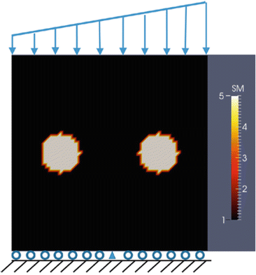
In the following we create hypothetical “measured” displacement data. In doing so, we define a square region of interest with unit length and a target shear modulus distribution consisting of two horizontally positioned inclusions in a homogeneous background (see Fig. 1). The shear modulus value in the inclusions is 5 and in the background 1. We apply a linear displacement boundary compression on the top edge, with the displacement varying from 0.002 to 0.008 from the left to right corner, respectively. The bottom edge is fixed in vertical direction and the center node on the bottom edge is fixed in all directions to prevent rigid body motion (see Fig. 1). All remaining boundary conditions not specified are traction free. The finite element mesh consists of 3,600 linear triangular elements and 3,721 mesh nodes. We add 3 % white Gaussian noise in order to mimic measured displacement data, which corresponds to about 70 % error in the strain field.


Fig. 1
Target shear modulus distribution of two inclusions in a homogeneous background. The bottom edge is fixed in vertical direction, represented by roller supports, except for the center node which is fixed in both directions. We apply a linearly varying compression on the top edge
2.2 Spatially Weighted Objective Function
In this section we present an alternative formulation of the objective function introduced in Sect. 2.1. We emphasize that the solution procedure of the inverse problem remains the same as discussed in Sect. 2.1. In order to simplify notations, we present the displacement correlation term in the objective function solely in terms of the vertical displacement component. We recall that we discard the horizontal displacement component entirely in the objective function. The modified objective function is given by

where u is the computed vertical displacement component and u meas is the measured vertical displacement component. W is a spatially weighted function defined as

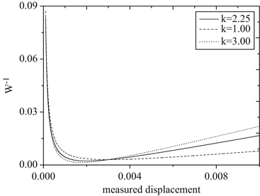
where u ave is the average measured displacement field of the entire region of interest, and b, k are constants. In Fig. 2 we plot the reciprocal of W over u meas for different choices of the parameter k. We note that for small measured displacements k does not change the curves significantly, while for increasing measured displacements the curves become increasingly steep with increasing values of k. We choose k such that the product of W(u measave)u measave is the same in both inclusions, where u measave is the average measured displacement in each inclusion. We determine the parameter  , the average measured displacement field in the entire region of interest
  , and set the parameter
  . From our experience, the solution of the inverse problem is not sensitive for a wide range of parameter choices for b. An explicit form is given by
  , where the index 1 and 2 refer to inclusion 1 and inclusion 2. In deriving the expression for k, we have assumed that b is much smaller than the averaged displacements, thus can be neglected.

(7)

(8)
 , the average measured displacement field in the entire region of interest
  , and set the parameter
  . From our experience, the solution of the inverse problem is not sensitive for a wide range of parameter choices for b. An explicit form is given by
  , where the index 1 and 2 refer to inclusion 1 and inclusion 2. In deriving the expression for k, we have assumed that b is much smaller than the averaged displacements, thus can be neglected.


