(1)
Department of Mathematics, University of Florida, Gainesville, FL, USA
4.1 Vector-Borne Diseases: An Introduction
A vector-borne disease is one in which the pathogenic microorganism is transmitted from an infected individual to another individual by an arthropod or other agent, sometimes with vertebrate animals serving as intermediary hosts. The transmission of vector-borne diseases to humans depends on three factors: (1) the pathogenic agent; (2) the arthropod vector; (3) and the human host. Mathematical models of vector-borne diseases typically take into account the dynamics of the vectors as well as the dynamics of the humans, and occasionally the dynamics of the intermediate animal host.
4.1.1 The Vectors
In epidemiology, a vector is a living carrier that transmits an infectious agent from one host to another. Vectors do not get ill from the disease, and once infected, they remain infected throughout the remainder of their lives. By common usage, vectors are considered to be invertebrate animals, usually arthropods. Technically, however, vertebrates can also act as vectors, including foxes, raccoons, and skunks, which can all transmit the rabies virus to humans via a bite. Arthropods account for over 85% of all known animal species, and they are the most important disease vectors. Examples of common vectors are mosquitoes, flies, sand flies, lice, fleas, ticks, mites, and cyclops, which transmit a huge number of diseases. Many such vectors feed on blood at some or all stages of their lives. When the arthropod feeds on blood, the parasite enters the blood stream of the host. Table 4.1 gives the most common vectors and the diseases they transmit.
Table 4.1
Examples of vectors and diseases they transmit
Vector | Diseases | Comment |
|---|---|---|
Flies | Bubonic plague | Flies |
Mosquitoes | Malaria | Anopheles genus |
Mosquitoes | Avian malaria, dengue, chikungunya | Aedes genus |
Tsetse flies | African sleeping sickness | Include 34 species of genus Glossina |
Kissing bugs | Chagas diseases | Triatominae subfamily of Reduviidae |
Ticks | Lyme disease, babesiosis | Genus Ixodes |
Sand flies | Leishmaniasis, bartonellosis, | Subfamily Phlebotominae |
sandfly fever | ||
Ticks, lice | Bacterial Rickettsia |
4.1.2 The Pathogen
The pathogen of the vector-borne diseases can fall in one of four categories:
Protozoa: A number of vector-borne diseases are caused by protozoa. The most notable example is malaria, which is caused by the Plasmodium parasite. The Plasmodium parasite has a complex life cycle that occurs in both the mosquito vector and the human host. Other vector-borne diseases caused by protozoa are trichomoniasis, leishmaniasis, and sleeping sickness.
Bacteria: Bacterial vector-borne diseases include Lyme disease, plague, tick-borne relapsing fever, and tularemia.
Virus: Most of the vector-borne diseases are caused by viruses. Most notable examples include dengue, chikungunya, eastern equine encephalitis, Japanese encephalitis, West Nile encephalitis, caused by the West Nile Virus, Yellow fever, and others. The viruses transmitted by arthropod vectors are known collectively as arboviruses.
Helminth: An example of a vector-borne disease cased by helminths (worms) is lymphatic filariasis, which is transmitted by mosquitoes.
4.1.3 Epidemiology of Vector-Borne Diseases
We summarize in Table 4.2 the primary examples of vector-borne diseases, the pathogens that cause them, the vectors that transmit them, and the human population at risk.
Table 4.2
Primary examples of vector-borne diseasesa
Population at | ||||
|---|---|---|---|---|
Disease | Pathogen | Vector | risk (millions) | Prevalence |
Malaria | Plasmodium spp. | Anopheles mosquito | 2100 | 270 million |
Schistosomiasis | Schistosome flatworms | Water snails | 600 | 260 million |
Dengue | Dengue virus | Aedes mosquitoes | 2000 | 50–100 million/yearb |
Leishmaniasis | Leishmania spp. | Sand flies | 12 | 350 million |
Lymphatic filariasis | Nematode worms | Mosquito | 900 | 65.5 million |
River blindness | Onchocerca volvulus | Black fly | 90 | 17.8 million |
African trypano- | Trypanosoma brucei spp. | Tsetse fly | 50 | 0.025 |
somiasis | million/year | |||
Chagas diseases | Trypanosoma cruzi spp. | Kissing bug | 100 | 6.5 million |
The majority of vector-borne diseases persist in nature by utilizing a vertebrate host. For a small number of vector-borne diseases, such as malaria and dengue, humans are the major host, with no significant animal reservoirs. The vector receives the pathogen from an infected host and transmits it either to an intermediary animal host or directly to the human host. The different stages of the pathogen’s life cycle occur during this process and are intimately dependent on the availability of suitable vectors and hosts.
Key components that determine the occurrence of vector-borne diseases include:
the abundance of vectors and intermediate and reservoir hosts;
the prevalence of disease-causing pathogens suitably adapted to the vectors and the human or animal host;
the local environmental conditions, especially temperature and humidity;
the resilience behavior and immune status of the human population.
Vector-borne diseases are prevalent in the tropics and subtropics and are relatively rare in temperate zones. Lyme disease and Rocky Mountain spotted fever persist in temperate regions, including the United States. There are different patterns of vector-borne disease occurrence. Parasitic and bacterial diseases, such as malaria and Lyme disease, tend to produce a high disease incidence but do not cause major outbreaks. An exception to this rule is plague, a bacterial disease that does cause outbreaks. In contrast, many vector viral diseases, such as yellow fever, dengue, and Japanese encephalitis, commonly cause major epidemics.
There has been a worldwide resurgence of vector-borne diseases since the 1970s, including malaria, dengue, yellow fever, plague, leishmaniasis, sleeping sickness, West Nile encephalitis, Lyme disease, Japanese encephalitis, Rift Valley fever, and Crimean-Congo hemorrhagic fever. Reasons for the emergence or resurgence of vector-borne diseases include:
the development of insecticide and drug resistance;
decreased resources for surveillance, prevention, and control of vector-borne diseases;
population growth;
urbanization;
changes in agricultural practices;
deforestation;
increased travel.
Changes in the distribution and population size of important arthropod disease vectors have also been observed. For instance,
The yellow fever mosquito, Aedes aegypti, has reestablished itself in parts of the Americas where it had been presumed to have been eradicated.
The Asian tiger mosquito, Aedes albopictus, was introduced into the Americas in the 1980s and has spread to Central and South America;
The black-legged tick, Ixodes scapularis, an important transmitter of Lyme disease and other pathogens, has gradually expanded its range in parts of eastern and central North America.
4.2 Simple Models of Vector-Borne Diseases
Historically, the first mathematical models of infectious diseases were derived at the beginning of the twentieth century. These models were developed by Ross and MacDonald to capture the dynamics of malaria and inform public health officials at that time how to combat malaria. Mathematical models of malaria have since become a guiding tool in the process of development and use of models in understanding infectious disease epidemiology and guiding control measures.
4.2.1 Deriving a Model of Vector-Borne Disease
Transmission in malaria, as in other vector-borne diseases, involves at least two species—the vector and the human host. The simplest model for the vector is an SI model, since most vectors once infected do not recover. Let us denote the susceptible vectors by S v and the infected vectors by I v . A susceptible vector becomes infected by biting an infected human I H at a biting rate a and probability of transmission of the disease given by p. The dynamical system that describes the vector is
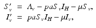
where  is the birth rate of the vectors, and μ is the death rate. Since the vectors such as the mosquito usually have a very short life cycle, demography should be included. The dynamics of the total vector population size
  is then given by the simplified logistic equation
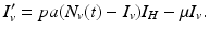
 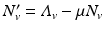 , whose solution can be obtained in explicit form. Since N v (t) is essentially a given function of t, we may express the number of susceptible vectors in terms of infected vectors
  and replace it in the second equation of system (4.1), thus essentially reducing the two-dimensional vector system to one equation:
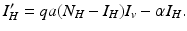
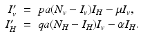
We turn now to the system for the humans. Humans generally recover from the disease, but for most vector-borne diseases, recovery is not permanent, and the recovered individual can become infected again. As a starting point, we model the transmission of a vector-borne disease in humans with an SIS model. Some of the vector-borne diseases, such as chikungunya, occur as outbreaks, and in this case, omitting births and deaths for humans is acceptable. Other vector-borne diseases, such as malaria, are endemic, and inclusion of demography in the human portion of the model is necessary. We begin with the simplest human model—an SIS model without demography. Susceptible humans in class S H become infected when bitten by an infectious vector. If we assume that infected vectors bite at the same rate as susceptible vectors, namely a, and q is the probability of transmission, then the model takes the form
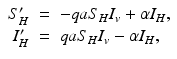
where α is the recovery rate. The total human population size N H is constant. We can reduce the human system by replacing the susceptible humans S H with 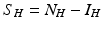 in the second equation. The system (4.3) reduces to the following equation:
The system for the infected vectors and infected humans becomes
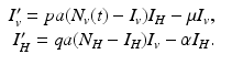
The right-hand side of this system depends on the unknown dependent variables I v and I H , and the known function of time N v (t). This makes the right-hand side explicitly dependent on time, and the model nonautonomous.
(4.1)
is the birth rate of the vectors, and μ is the death rate. Since the vectors such as the mosquito usually have a very short life cycle, demography should be included. The dynamics of the total vector population size is then given by the simplified logistic equation , whose solution can be obtained in explicit form. Since N v (t) is essentially a given function of t, we may express the number of susceptible vectors in terms of infected vectors and replace it in the second equation of system (4.1), thus essentially reducing the two-dimensional vector system to one equation:(4.2)
(4.3)
in the second equation. The system (4.3) reduces to the following equation:(4.4)
(4.5)
Definition 4.1.
A differential equation model y′ = f(t, y) is called nonautonomous if the right-hand-side function f(t, y) depends explicitly on t.
Nonautonomous models are harder to analyze and are often not subjected to the rules of autonomous models that we investigate in this book. However, system (4.5) depends on time only through the function N v (t), which has a limit as time goes to infinity, namely,
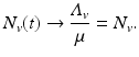
Suppose we replace system (4.5) with the following limiting system:
The limiting system (4.6) is an autonomous system, which is easier to analyze. Nonautonomous models whose limiting system is an autonomous model are called asymptotically autonomous.
(4.6)
The main question that remains is whether the global dynamics of system (4.6) are similar to the dynamics of the original nonautonomous system (4.5). If the answer is yes, then we may investigate system (4.6), for which a number of tools exist, and draw conclusions about system (4.5). The following theorem gives a positive answer to this question for planar systems.
Theorem 4.1 (Thieme [150]).
Assume that x′ = f(t,x) is a nonautonomous system such that x ∈ R 2 and y′ = g(y) is the limiting autonomous system. Let ω be the ω-limit set of a forward bounded solution x of the nonautonomous system. Assume that there exists a neighborhood of ω that contains at most finitely many equilibria of the autonomous system. Then the following trichotomy holds:
1.
ω consists of an equilibrium of the autonomous system.
2.
ω is a union of periodic orbits of the autonomous system and possible centers that are surrounded by periodic orbits of the autonomous system lying in ω.
3.
ω contains equilibria of the autonomous system that are cyclically chained to each other in ω by orbits of the autonomous system.
First, we show that all solutions of the nonautonomous system (4.5) are bounded. Indeed, suppose for some t ∗ that I v (t ∗) > N v (t ∗). Then I v ′(t ∗) < 0, and I v (t) is decreasing for all t for which it exceeds N v (t). Hence, 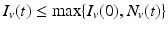 . Similar reasoning shows that I H (t) is bounded.
. Similar reasoning shows that I H (t) is bounded.Since all solutions of the nonautonomous system (4.5) are bounded, the above theorem implies that the ω-limit set of the nonautonomous system can be obtained from investigation of the ω-limit set of the autonomous system (4.6). We focus on the investigation of the global behavior of the solutions of system (4.6).
System (4.6) is often recast in terms of proportions. If we set  and
and  , then the system for the proportions becomes
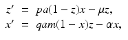
where  is the proportion of vectors to humans, and a has absorbed a multiple of the total human population.
and , then the system for the proportions becomes(4.7)
is the proportion of vectors to humans, and a has absorbed a multiple of the total human population.4.2.2 Reproduction Numbers, Equilibria, and Their Stability
We will derive reproduction numbers and the equilibria for the original dimensional system (4.6). To compute equilibria, we set the system equal to zero:
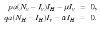
The system clearly has the disease-free equilibrium  . To compute the reproduction number and investigate the stability of the disease-free equilibrium, we consider the Jacobian of the system (4.6):
The disease-free equilibrium is stable if 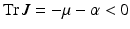 , which is clearly satisfied, and also if
  , gives the reproduction number of a vector-borne disease, where
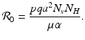 We see that the local stability/instability of the disease-free equilibrium is connected to the basic disease reproduction number
  , which identifies the threshold for the local stability of the disease-free equilibrium. The disease-free equilibrium is locally asymptotically stable (the disease dies out) if
  , and unstable if
 ![$$\mathcal{R}_{0} > 1$$
” src=”/wp-content/uploads/2016/11/A304573_1_En_4_Chapter_IEq16.gif”></SPAN>. This is a critical parameter for control of the disease, since if <SPAN id=IEq17 class=InlineEquation><IMG alt=]() 1$$
” src=”/wp-content/uploads/2016/11/A304573_1_En_4_Chapter_IEq17.gif”>, introduction of a small amount of disease into the population may cause it to evolve into an endemic prevalence.
1$$
” src=”/wp-content/uploads/2016/11/A304573_1_En_4_Chapter_IEq17.gif”>, introduction of a small amount of disease into the population may cause it to evolve into an endemic prevalence.
(4.8)
. To compute the reproduction number and investigate the stability of the disease-free equilibrium, we consider the Jacobian of the system (4.6):(4.9)
, which is clearly satisfied, and also if , gives the reproduction number of a vector-borne disease, where, which identifies the threshold for the local stability of the disease-free equilibrium. The disease-free equilibrium is locally asymptotically stable (the disease dies out) if , and unstable if The disease reproduction number  is one of the main epidemiological indicators of whether a disease can successfully invade and persist in a population. In vector-borne diseases, just as in directly transmitted diseases, the disease reproduction number gives the number of secondary infections of humans that one infective human individual may produce in a population of susceptible human individuals. The classical approach of Kermack and McKendrick derives
  from the condition for local stability of the disease-free equilibrium. Other approaches are possible, and will be discussed later.
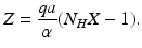
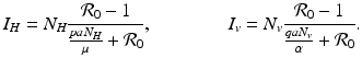
is one of the main epidemiological indicators of whether a disease can successfully invade and persist in a population. In vector-borne diseases, just as in directly transmitted diseases, the disease reproduction number gives the number of secondary infections of humans that one infective human individual may produce in a population of susceptible human individuals. The classical approach of Kermack and McKendrick derives from the condition for local stability of the disease-free equilibrium. Other approaches are possible, and will be discussed later.Transmission of vector-borne diseases involves two transmission cycles, namely human to vector and vector to human, and each of these transmission processes may be characterized by its own disease reproduction number. These two numbers may be combined to form a single dimensionless number that indicates whether, and to some extent how seriously, the human–vector system is open to invasion by the parasite. The Kermack–McKendrick–MacDonald approach places one infected human in a population of susceptible vectors; there will result  secondary infected vectors. Similarly, placing one infected vector in a population of susceptible humans will produce
  infected humans, where
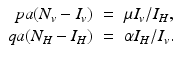
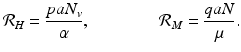 To understand these definitions, consider the incidence term in the equation for the vectors pa(N v − I v )I H , which gives the number of secondary infections of vectors I H infected humans will produce per unit of time. Then, one infected human will produce paN v infected vectors in an entirely susceptible vector population per unit of time. One infected human is infectious for 1∕α time units; hence we obtain
  . Similar reasoning leads to
  . To account for the secondary human infections that one infected human will produce, we notice that one infected human will produce
  infected vectors, each of which will produce
  infected humans, giving
 secondary human infections. This expression gives the classical reproduction number of vector-borne diseases.
secondary infected vectors. Similarly, placing one infected vector in a population of susceptible humans will produce infected humans, where. Similar reasoning leads to . To account for the secondary human infections that one infected human will produce, we notice that one infected human will produce infected vectors, each of which will produce infected humans, givingTo compute the endemic equilibrium, we consider again system (4.8). This system is nonlinear in I v and I H and not easy to solve directly. To simplify the solution, we adopt the substitution  ,
,  , which transforms the system into a linear inhomogeneous system of equations for X and Z:
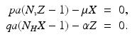
, , which transforms the system into a linear inhomogeneous system of equations for X and Z:(4.10)
Solving this linear system, we obtain
 Substituting Z in the first equation and solving for X, we obtain X in terms of the parameter values. Further substituting X in the equation for Z, we obtain the following equilibrium:
From these expressions, it is clear that the endemic equilibrium exists and is positive if and only if ![$$\mathcal{R}_{0} > 1$$
” src=”/wp-content/uploads/2016/11/A304573_1_En_4_Chapter_IEq28.gif”></SPAN>. From the expressions above, we can easily compute the values of the equilibrium for the proportions <SPAN class=EmphasisTypeItalic>x</SPAN> and <SPAN class=EmphasisTypeItalic>z</SPAN>.</DIV><br />
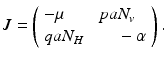
<DIV class=Para>Next, we investigate the local stability of the endemic equilibrium. This can be obtained from the Jacobian matrix at the endemic equilibrium, which is obtained from the linearization of system (<SPAN class=InternalRef><A href=]() 4.6) around the endemic equilibrium. The Jacobian is given by the matrix
4.6) around the endemic equilibrium. The Jacobian is given by the matrix
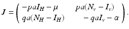
The trace of the matrix is negative: 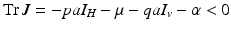 . To determine the sign of the determinant, notice that
From these equations, it follows that 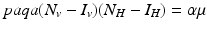 . This identity simplifies the determinant of the Jacobian and helps determine its sign:
  , which takes the form
(4.11)
(4.12)
. To determine the sign of the determinant, notice that(4.13)
. This identity simplifies the determinant of the Jacobian and helps determine its sign: , which takes the form


