The SIR Model with Demography: General Properties of Planar Systems

(1)

Department of Mathematics, University of Florida, Gainesville, FL, USA

3.1 Modeling Changing Populations

Models that do not explicitly include births and deaths occurring in the population are called epidemic models without explicit demography. They are useful for epidemic modeling on a short time scale, particularly for modeling epidemic outbreaks such as influenza. Omitting population change requires that the disease develop on a much shorter time scale than the period in which significant change in the population size can occur (such as births and deaths). This is valid for fast diseases like the childhood diseases and influenza. On the other hand, there are slow diseases, such as HIV, tuberculosis, and hepatitis C, that develop for a long period of time even on an individual level. In this case, the total population does not remain constant for long periods of time, and the demography of the population cannot be ignored.

To incorporate the population change in epidemic models, we need population models of the growth of the human population. There are several classical population models that are typically considered in the literature.

Population growth is the rate of change in a population over time, and it can be approximated as the change in the number of individuals of any species in a population per unit time. The study of growth and change of human populations is called demography. Modeling and projecting the growth of human populations is in general not a simple matter, but for the purposes of epidemic modeling, we will use several simple population models.

3.1.1 The Malthusian Model

The Malthusian model, sometimes called the exponential model, is essentially an exponential growth model based on the assumption that the rate of change of a population is proportional to the total population size. The model is named after the Reverend Thomas Malthus (1766–1834), who authored An Essay on the Principle of Population, one of the earliest and most influential books on populations. The Malthusian model is based on the following assumptions: (1) All individuals are identical, that is, they are not classified by age, sex, or other characteristics. (2) The environment is constant in space and time, in particular, resources are unlimited. With these assumptions, if N(t) is the total population size, and b is the per capita birth rate, while μ is the per capita death rate, then the Malthusian model becomes

$\displaystyle{ N'(t) = bN(t) -\mu N(t) = rN(t), }$

(3.1)

where r = b −μ is the population growth rate. The solution to this equation is an exponential N(t) = N(0)e ^rt. The population is growing exponentially if r > 0, decreasing exponentially if r < 0, and constant if r = 0.

We compare the performance of population models with world population data. Table 3.1 gives the world’s human population since 1950.

Table 3.1

World population size 1950–2010^a

Year	Population	Year	Population
1950	2,556,505,579	1980	4,452,686,744
1952	2,635,724,824	1982	4,615,366,900
1954	2,729,267,486	1984	4,776,577,665
1956	2,834,435,383	1986	4,941,825,082
1958	2,947,380,005	1988	5,114,949,044
1960	3,042,389,609	1990	5,288,828,246
1962	3,139,645,212	1992	5,456,405,468
1964	3,280,890,090	1994	5,619,031,095
1966	3,420,438,740	1996	5,779,990,768
1968	3,562,227,755	1998	5,935,741,324
1970	3,712,813,618	2000	6,088,683,554
1972	3,867,163,052	2002	6,241,717,680
1974	4,017,615,739	2004	6,393,120,940
1976	4,161,423,905	2006	6,545,884,439
1978	4,305,496,751	2008	6,700,765,879
–	–	2010	6,853,019,414

^a Data taken from http://www.census.gov/ipc/www/idb/worldpop.php

With the simple population models in this section, many methods for estimating the parameters can work. One of the most powerful methods, however, is calibration or curve fitting. Curve fitting is the process of identifying the parameters of a curve, or mathematical function, that has the best fit to a series of data points. We discuss more thoroughly fitting epidemic models to data in Chap. 6 Here we only compare the population models with the available data.

Calibration is greatly expedited through the use of software such as Mathematica, Matlab, or R to fit the model to the data. For the Malthusian model, we have an explicit solution, and we can fit the solution function to the data. Since the initial condition for the data is not at zero, the solution to the Malthus model becomes N(t) = Ae ^r(t−1950). We fit both A and r. Fitting in Mathematica can be done with the command NonlinearModelFit. The result of the fit of the world population data to the Malthusian model is given in Fig. 3.1, where the population is taken in millions.

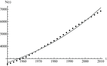
Fig. 3.1

World population data alongside Malthusian model predictions. The estimated values of the parameters are A = 2676. 29 and r = 0. 0163. The least-squares error of the fit is E = 402, 533

3.1.2 The Logistic Model as a Model of Population Growth

The Malthus model assumes that the population’s per capita growth rate is constant and that the population has unlimited resources by which to grow. In most cases, however, populations live in an environment that has a finite capacity to support only a certain population size. When the population size approaches this capacity, the per capita growth rate declines or becomes negative. This property of the environment to limit population growth is captured by the logistic model. The logistic model was developed by the Belgian mathematician Pierre Verhulst (1838), who suggested that the per capita growth rate of the population may be a decreasing function of population density:

$\displaystyle{ \frac{1} {N(t)}N'(t) = r\left (1 -\frac{N} {K}\right ),}$

which gives the classical logistic model that we studied in Chap. 2 At low densities N(t) ≈ 0, the population growth rate is maximal and equals r. The parameter r can be interpreted as the population growth rate in the absence of intraspecific competition. The population growth rate declines with population number N and reaches 0 when N = K. The parameter K is the upper limit of population growth, and it is called the carrying capacity of the environment. It is usually interpreted as the quantity of resources expressed in the number of organisms that can be supported by those resources. If population number exceeds K, then population growth rate becomes negative, and population declines. The logistic model has been used unsuccessfully for the projection of human populations. The main difficulty appears to be determining the carrying capacity of a human population. It is believed that human populations do not have a carrying capacity, and even if they do, that the carrying capacity is not constant. For those reasons, the logistic model is rarely used to model human populations. However, when compared to population data, the logistic equation usually performs admirably in modeling the data for short periods of time. We use the logistic model to model the world population data. The results are given in Fig. 3.2.

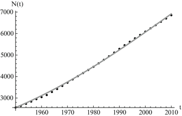
Fig. 3.2

World population data alongside logistic model predictions. The estimated values of the parameters are K = 13, 863. 9 and r = 0. 0247. The least-squares error of the fit is E = 56, 659. 3

3.1.3 A Simplified Logistic Model

The third model of population growth is a simplified version of the logistic model. It assumes constant birth rate, independent of population size. It also assumes constant per capita death rate. The model becomes

$\displaystyle{N'(t) =\varLambda -\mu N.}$

Here $\varLambda$ is the total birth rate, and μ is the per capita natural death rate. Then μ N is the total death rate. This model can be solved. The solution is

$\displaystyle{N(t) = N_{0}e^{-\mu t} + \frac{\varLambda } {\mu }(1 - e^{-\mu t}).}$

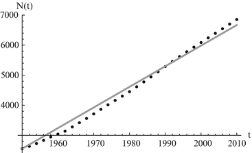
It is not hard to see that if $t \rightarrow \infty$ , then $N(t) \rightarrow \frac{\varLambda }{\mu }$ . This limit quantity is called the limit population size. The simplified logistic model is the one most often used to model population dynamics in epidemic models. However, its performance with data is modest. We illustrate how the simplified logistic model fits the world population data in Fig. 3.3.

Fig. 3.3

World population data alongside the simplified logistic model predictions. The estimated values of the parameters are μ = 5. 54 × 10⁻¹² and $\varLambda = 68.5$ , and we have preset N(1950) = 2556. 5. The least-squares error of the fit is E = 703, 482

We saw in Chap. 2 that if T is the time spent is a class (or a compartment), then the per capita rate at which the individuals leave that class (compartment) is given by $\frac{1} {T}$ . So if the per capita recovery rate was α, then

$\displaystyle{\alpha = \frac{1} {T},}$

or equivalently, $\frac{1} {\alpha }$ is the time spent in the infectious compartment. Similar reasoning can be applied to the compartment “life.” If μ is the natural death rate, then 1∕μ should be the average lifespan of an individual human being. From fitting the simplified logistic model to world data, we estimated μ = 5. 54 × 10⁻¹², which gives a lifespan of 1. 8 × 10¹¹ years—quite unrealistic. If the lifespan is limited to biologically realistic values, such as a lifespan of 65 years, then the fit becomes worse.

3.2 The SIR Model with Demography

To incorporate the demographics into the SIR epidemic model, we assume that all individuals are born susceptible. Individuals from each class die at a per capita death rate μ, so the total death rate in the susceptible class is μ S, while in the infective class, it is μ I, and in the removed class, it is μ R. The epidemic model with demography becomes

$\displaystyle\begin{array}{rcl} S'(t)& =& \varLambda -\beta IS -\mu S, \\ I'(t)& =& \beta IS -\alpha I -\mu I, \\ R'(t)& =& \alpha I -\mu R. {}\end{array}$

(3.2)

We add the three equations to obtain the total population. The model of the total population is $N'(t) =\varLambda -\mu N$ , where N = S + I + R. The population size is not constant, but it is asymptotically constant, since $N(t) \rightarrow \frac{\varLambda }{\mu }$ as $t \rightarrow \infty$ .

When the population is nonconstant and the incidence is proportional to the product of I and S, we say that the incidence is given by the law of mass action, analogously to terms from chemical kinetic models, whereby chemicals react by bumping randomly into each other. For this reason, this incidence is called the mass action incidence:

mass action incidence = β S I.

Another type of incidence that is very commonly used in epidemic models is the standard incidence. It is similar to the mass action incidence, but it is normalized by the total population size. In particular,

standard incidence = $\frac{\beta SI} {N}$ .

The mass action incidence and the standard incidence agree when the total population size is a constant, but they differ if the total population size is variable. Mass action incidence is used in diseases for which disease-relevant contact increases with an increase in the population size. For instance, in influenza and SARS, contacts increase as the population size (and density) increase. Standard incidence is used for diseases for which the contact rate cannot increase indefinitely and is limited even if the population size increases. This is the case in sexually transmitted diseases, where the number of contacts cannot increase indefinitely.

We notice as before that the first two equations in (3.2) are independent of the third, and we consider the two-dimensional system

$\displaystyle\begin{array}{rcl} S'(t)& =& \varLambda -\beta IS -\mu S, \\ I'(t)& =& \beta IS -\alpha I -\mu I,{}\end{array}$

(3.3)

where R = N − S − I. Mathematically, the SIR system can be written in the general form

$\displaystyle\begin{array}{rcl} S'(t)& =& f(S,I), \\ I'(t)& =& g(S,I).{}\end{array}$

(3.4)

This is a system of differential equations with two equations and the two unknowns S and I. The incidence term makes both f and g nonlinear functions. So system (3.4) is a nonlinear system of differential equations. System (3.4) is also autonomous, since f and g do not depend explicitly on the time variable; that is, the coefficients of system (3.3) are constants and not functions of time.

What are the units of the quantities in this model? Since S is measured in number of people, it follows that S′ is measured in number of people per unit of time. The total birth rate $\varLambda$ is measured in number of people born per unit of time. The per capita death rate μ is measured in [unit of time]⁻¹. Thus, μ S is measured again in number of people per unit of time. The most difficult term is β I S. Since the force of infection β I is a per capita rate, it has units [time]⁻¹. Consequently, the transmission coefficient β must have units of [number of people× time]⁻¹.

A customary transformation of the system (3.3) that simplifies the system and reduces the number of parameters is often performed. There is a simplification that consists in a change of variables that transforms both the independent variable and the dependent variables into nondimensional quantities. Hence, we say that we have transformed the system into a nondimensional form.

Two parameters have units [unit of time]⁻¹: α and μ. Since t is in [unit of time], we have to multiply t by one of the rates to obtain a unitless quantity. It is best to define τ = (α +μ)t. Observe that τ is a dimensionless quantity. Because of the nature of the change, this change will remove the parameter multiplying I. Let $N(t) = N( \frac{\tau }{\alpha +\mu }) =\hat{ N}(\tau )$ . Similarly, $I(t) =\hat{ I}(\tau )$ . By the chain rule, we have

$\displaystyle{ \begin{array}{l} \frac{d\hat{S}} {d\tau } = \frac{1} {\alpha +\mu } \frac{dS} {dt}, \\ \frac{d\hat{I}} {d\tau } = \frac{1} {\alpha +\mu } \frac{dI} {dt}. \\ \end{array} }$

(3.5)

We rescale the $\hat{S}$ and $\hat{I}$ variables with the total limiting population size. Hence $x(t) = \frac{\mu \hat{S}} {\varLambda }$ and $y(t) = \frac{\mu \hat{I}} {\varLambda }$ . The new dependent variables x(τ) and y(τ) are also dimensionless quantities. The system for them becomes

$\displaystyle{ \begin{array}{l} x' =\rho (1 - x) -\mathcal{R}_{0}xy, \\ y' = (\mathcal{R}_{0}x - 1)y,\end{array} }$

(3.6)

where

$\displaystyle{\rho =\mu /(\alpha +\mu )\qquad \qquad \mathcal{R}_{0} = \frac{\varLambda \beta } {\mu (\alpha +\mu )}}$

are both dimensionless parameters. The notation $\mathcal{R}_{0}$ is not random. As we will see later, this dimensionless quantity is indeed the reproduction number. Notice that we have reduced the number of parameters from five to two. The dimensionless form of the SIR model with demography is equivalent to the original one, since the solutions of both systems have the same long-term behavior.

3.3 Analysis of Two-Dimensional Systems

We cannot solve the SIR model with demography analytically, but we can obtain some information about the behavior of the solutions. The long-term behavior of the solutions is particularly important from an epidemiological perspective, since we would like to know what will happen to the disease in the long run: will it die out, or will it establish itself in the population and become endemic?

3.3.1 Phase-Plane Analysis

We write the system (3.6) in general form

$\displaystyle{ \begin{array}{l} x' = f(x,y), \\ y' = g(x,y),\end{array} }$

(3.7)

where $f(x,y) =\rho (1 - x) -\mathcal{R}_{0}xy$ and $g(x,y) = (\mathcal{R}_{0}x - 1)y$ . To answer the question above, we have to investigate the long-term behavior of the solutions. Instead of considering x(τ) and y(τ) as functions of τ, or equivalently, S(t) and I(t) as functions of t, we treat τ as a parameter and consider the curves in the (x, y)-plane, obtained from the points (x(τ), y(τ)) as τ varies as a parameter. By considering the solution curves in the (x, y)-plane, we say that we are considering the phase plane.

Definition 3.1.

Curves in the phase plane representing the functional relation between x and y, with τ as a parameter, are called orbits or trajectories.

The long-term behavior of the trajectories depends largely on the equilibrium points, that is, on time-independent solutions of the system. Equilibrium points are solutions for which x′ = 0 and y′ = 0.

Definition 3.2.

All points (x ^∗, y ^∗), where x ^∗ and y ^∗ are constants that satisfy the system

$\displaystyle\begin{array}{rcl} f(x^{{\ast}},y^{{\ast}})& =& 0, \\ g(x^{{\ast}},y^{{\ast}})& =& 0,{}\end{array}$

(3.8)

are called equilibria or singular points.

For the dimensionless SIR model with demography, we have

$\displaystyle\begin{array}{rcl} \rho (1 - x) -\mathcal{R}_{0}xy& =& 0, \\ (\mathcal{R}_{0}x - 1)y& =& 0.{}\end{array}$

(3.9)

We have that if y = 0, that is, there are no infectives, then x = 1; that is, everyone is susceptible. This gives the first equilibrium in the (x, y)-plane, (1, 0). This is the disease-free equilibrium. The disease-free equilibrium is also a boundary equilibrium, since it lies on the boundary of the feasible region x ≥ 0, y ≥ 0. If y ≠ 0, then from the second equation, we have $x = 1/\mathcal{R}_{0}$ . From the first equation, we have $y =\rho (1 - 1/\mathcal{R}_{0})$ . Thus the second equilibrium is the point

$\displaystyle{\mathcal{E} = \left ( \frac{1} {\mathcal{R}_{0}},\rho \left (1 - \frac{1} {\mathcal{R}_{0}}\right )\right ).}$

This is the endemic equilibrium. The endemic equilibrium exists only in the case $$$\mathcal{R}_{0} > 1$$ ” src=”/wp-content/uploads/2016/11/A304573_1_En_3_Chapter_IEq23.gif”>. This equilibrium is also called an interior equilibrium.</DIV> <DIV class=Para>System (<A href=$ 3.6) allows us to compute the slope at each point of a trajectory in the (x, y)-plane. The parameter τ can be eliminated by dividing the equations in system (3.6):

$\displaystyle{\frac{dy} {dx} = \frac{g(x,y)} {f(x,y)}.}$

This quotient is defined for all points in the (x, y)-plane except the equilibria. For any nonequilibrium point (x ₀, y ₀) in the phase plane, we can compute the expression

$\displaystyle{\frac{dy} {dx}\vert _{(x_{0},y_{0})} = \frac{g(x,y)} {f(x,y)}}$

which gives the slope of the trajectory in the (x, y)-plane, with tangent vector

$\displaystyle{(f(x_{0},y_{0}),g(x_{0},y_{0}))^{T}.}$

This vector also gives the direction of the trajectory. The tangent vector is not defined at the equilibria, since the flow stops at those points and they are fixed points.

Fig. 3.4

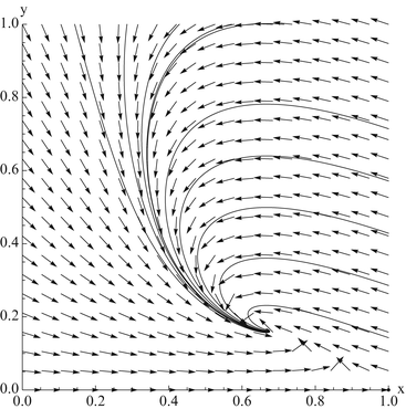
The vector field of the dimensionless SIR model alongside solutions of the model for several initial conditions

The collection of tangent vectors defines a direction field. The direction field can be used as a visual aid in sketching a family of solutions called a phase-plane portrait or a phase-plane diagram. A phase-plane portrait of the dimensionless SIR model is given in Fig 3.4. The creation of the whole phase portrait is a tedious job and is done only by computer. An easier method to obtain information about the direction of the flow is to analyze the direction of the flow along the x-zero and y-zero isoclines, or nullclines.

Definition 3.3.

The x-zero isocline or x-nullcline for the system (3.7) is the set of all points in the (x, y)-plane satisfying

$\displaystyle{f(x,y) = 0.}$

The y-zero isocline or y-nullcline for the system (3.7) is the set of all points in the (x, y)-plane satisfying

$\displaystyle{g(x,y) = 0.}$

We can determine the nullclines for the dimensionless SIR model. Setting $\rho (1 - x) -\mathcal{R}_{0}xy = 0$ gives the x-nullcline

$\displaystyle{y = \frac{\rho } {\mathcal{R}_{0}} \frac{1 - x} {x}.}$

Setting $(\mathcal{R}_{0}x - 1)y = 0$ gives two y-nullclines: y = 0, which is the x-axis, and the vertical line $x = \frac{1} {\mathcal{R}_{0}}$ . The points where an x-nullcline intersects a y-nullcline give the equilibrium points of the system. There are two scenarios for the SIR dimensionless system.

$\mathcal{R}_{0} < 1$

In this case, there is only one intersection of an x-nullcline and a y-nullcline. The x-nullcline intersects the y-nullcline y = 0 at the point (1, 0), the disease-free equilibrium. Since $$$1/\mathcal{R}_{0} > 1$$ ” src=”/wp-content/uploads/2016/11/A304573_1_En_3_Chapter_IEq29.gif”>, the y-nullcline <IMG alt=$ does not intersect the x-nullcline in the positive quadrant.

$$$\mathcal{R}_{0} > 1$$ ” src=”/wp-content/uploads/2016/11/A304573_1_En_3_Chapter_IEq31.gif”> <DIV class=Description> <DIV class=Para>In this case, there are two intersections of an x-nullcline and a y-nullcline. In the first intersection, the x-nullcline intersects the y-nullcline y = 0 at the point (1, 0), which represents the disease-free equilibrium. In the second intersection, since <IMG alt=$ , the y-nullcline $x = 1/\mathcal{R}_{0}$ intersects the x-nullcline $1/\mathcal{R}_{0} < 1$ at the point $\mathcal{E}$ , which gives the endemic equilibrium.

To determine the direction of the vector field along the nullclines, we can use the following general rules:

On the x-nullclines, the tangent vector is

$\displaystyle{(0,g(x_{0},y_{0}))^{T}}$

and is parallel to the y-axis. The direction of the tangent is given by the sign of g(x ₀, y ₀). If g(x ₀, y ₀) > 0, the direction vector points upward. If g(x ₀, y ₀) < 0, the directional vector points downward.

On the y-nullclines, the tangent vector is

$\displaystyle{(f(x_{0},y_{0}),0)^{T}}$

and is parallel to the x-axis. The direction of the tangent vector is determined by the sign of f(x ₀, y ₀). If f(x ₀, y ₀) > 0, the direction vector points to the right. If f(x ₀, y ₀) < 0, the direction vector points to the left.

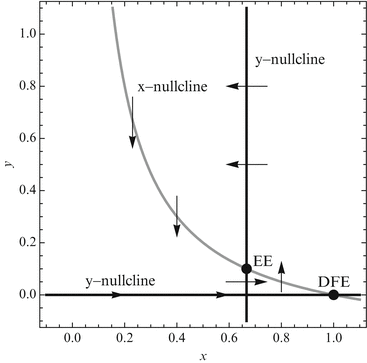
We determine the direction field along nullclines for the dimensionless SIR model. We consider the case $$$\mathcal{R}_{0} > 1$$ ” src=”/wp-content/uploads/2016/11/A304573_1_En_3_Chapter_IEq36.gif”>. The case <IMG alt=$ is similar. The results are illustrated in Fig. 3.5.

Fig. 3.5

Phase-plane analysis of the dimensionless SIR model. Nullclines and the direction of the vector field along them

On the x-nullcline, the tangent vector is (0, g(x ₀, y ₀))^T, where (x ₀, y ₀) is a point on the nullcline. The tangent vector is parallel to the y-axis. Since $g(x_{0},y_{0}) = (\mathcal{R}_{0}x_{0} - 1)y_{0}$ and y ₀ > 0, the sign of g(x ₀, y ₀) is determined by the first term in the product. Thus, if $x_{0} < 1/\mathcal{R}_{0}$ , then g(x ₀, y ₀) < 0, and the vector points downward. If $$$x_{0} > 1/\mathcal{R}_{0}$$ ” src=”/wp-content/uploads/2016/11/A304573_1_En_3_Chapter_IEq40.gif”>, then g(x 0, y 0) > 0, and the vector points upward.</DIV></DIV> <DIV class=ClearBoth> </DIV></DIV> <DIV class=ListItem>2. <DIV class=ItemContent> <DIV class=Para>On the y-nullclines, the tangent vector is (f(x 0, y 0), 0) T , where (x 0, y 0) is a point on a y-nullcline. The tangent vector is parallel to the x-axis. Since there are two y-nullclines, we consider two cases: <DIV class=DefinitionList> <DIV class=DefinitionListEntry>y = 0 <DIV class=Description> <DIV class=Para>On the nullcline y = 0, f(x 0, y 0) = ρ(1 − x 0). We have f(x 0, y 0) > 0 if x 0 < 1, and the tangent vector points to the right. Furthermore, we have f(x 0, y 0) < 0 if x 0 > 1, and the tangent vector points to the left.</DIV></DIV></DIV> <DIV class=DefinitionListEntry><IMG alt=$

On the y-nullcline $x = \frac{1} {\mathcal{R}_{0}}$ , we have $f(x_{0},y_{0}) =\rho \left (1 - \frac{1} {\mathcal{R}_{0}} \right ) - y_{0}$ . We have that $$$y_{0} >\rho \left (1 – \frac{1} {\mathcal{R}_{0}} \right )$$ ” src=”/wp-content/uploads/2016/11/A304573_1_En_3_Chapter_IEq45.gif”> if the point (x 0, y 0) is on the y-nullcline above the intersection of the y-nullcline with the x-nullcline. Hence, f(x 0, y 0) < 0, and the tangent vector points to the left. Furthermore, we have that <IMG alt=$ if the point (x ₀, y ₀) is on the y-nullcline below the intersection of the y-nullcline with the x-nullcline. Hence, f(x ₀, y ₀) > 0, and the tangent vector points to the right.

3.3.2 Linearization

Just as with first-order nonlinear equations, we can obtain information about the behavior of the solutions near an equilibrium through linearization. If (x ^∗, y ^∗) is an equilibrium, we consider the perturbation of a solution starting from an initial condition close to the equilibrium:

$\displaystyle{u(\tau ) = x(\tau ) - x^{{\ast}}\qquad \qquad v(\tau ) = y(\tau ) - y^{{\ast}}.}$

We note again that u(τ) and v(τ) are functions of τ but are not necessarily nonnegative. Writing x(τ) = u(τ) + x ^∗, y(τ) = v(τ) + y ^∗, and substituting in the original system, we obtain

$\displaystyle{ \begin{array}{l} u' = f(u + x^{{\ast}},v + y^{{\ast}}), \\ v' = g(u + x^{{\ast}},v + y^{{\ast}}).\end{array} }$

(3.10)

Assuming that f and g have at least second-order continuous partial derivatives, we expand in a Taylor series using the theorem for functions of two variables. We show that expansion for f; the process for g is the same.

$\displaystyle\begin{array}{rcl} f(u + x^{{\ast}},v + y^{{\ast}})& =& f(x^{{\ast}},y^{{\ast}}) + f_{ x}(x^{{\ast}},y^{{\ast}})u(\tau ) + f_{ y}(x^{{\ast}},y^{{\ast}})v(\tau ) \\ & & +f_{xx}(x^{{\ast}},y^{{\ast}})u^{2}(\tau )/2 + f_{ xy}(x^{{\ast}},y^{{\ast}})u(\tau )v(\tau ) \\ & & +f_{yy}(x^{{\ast}},y^{{\ast}})v^{2}(\tau )/2 + \cdots \,. {}\end{array}$

(3.11)

The terms with the second partial derivatives are multiplied by u ², uv, and v ², all second-order terms in the perturbations. If the perturbations are small, u ≈ 0 and v ≈ 0, then the second-order terms are even smaller, so we may ignore them. Thus,

$\displaystyle{ \begin{array}{l} u' \approx f(x^{{\ast}},y^{{\ast}}) + f_{x}(x^{{\ast}},y^{{\ast}})u(\tau ) + f_{y}(x^{{\ast}},y^{{\ast}})v(\tau ), \\ v' \approx g(x^{{\ast}},y^{{\ast}}) + g_{x}(x^{{\ast}},y^{{\ast}})u(\tau ) + g_{y}(x^{{\ast}},y^{{\ast}})v(\tau ).\end{array} }$

(3.12)

Since (x ^∗, y ^∗) is an equilibrium, f(x ^∗, y ^∗) = 0 and g(x ^∗, y ^∗) = 0. We obtain the linearized system

$\displaystyle{ \begin{array}{l} u' = f_{x}(x^{{\ast}},y^{{\ast}})u(\tau ) + f_{y}(x^{{\ast}},y^{{\ast}})v(\tau ), \\ v' = g_{x}(x^{{\ast}},y^{{\ast}})u(\tau ) + g_{y}(x^{{\ast}},y^{{\ast}})v(\tau ). \end{array} }$

(3.13)

The matrix of the partial derivatives of the functions f(x, y) and g(x, y) is called the Jacobian matrix. The matrix of the system above is the Jacobian matrix evaluated at an equilibrium (x ^∗, y ^∗). All entries of this matrix are given constants:

$\displaystyle{ J = \left (\begin{array}{l} f_{x}(x,y)\qquad f_{y}(x,y) \\ g_{x}(x,y)\qquad g_{y}(x,y) \end{array} \right )\vert _{x=x^{{\ast}},y=y^{{\ast}}} }$

(3.14)

An important result, called the Hartman–Grobman theorem justifies drawing conclusions about a nonlinear system from studying the linearized system. The Hartman–Grobman theorem says roughly that the solutions of an n × n autonomous system of ordinary differential equations in a neighborhood of a steady state look “qualitatively” just like the solutions of the linearized system (3.13) near the point (0, 0). This result holds only when the equilibrium is a hyperbolic equilibrium, that is, when none of the eigenvalues of J have zero real part.

3.3.3 Two-Dimensional Linear Systems

The linearized system (3.13) can be written in the form

$\displaystyle\begin{array}{rcl} u'& =& au(\tau ) + bv(\tau ), \\ v'& =& cu(\tau ) + dv(\tau ),{}\end{array}$

(3.15)

where a, b, c, d are given constants. The system (3.15) is a two-dimensional linear homogeneous system. The behavior of solutions of such systems has been completely studied. In this subsection, we review what is known about two-dimensional linear systems. The equilibria of linear two-dimensional systems are solutions to the linear system of equations

$\displaystyle\begin{array}{rcl} au(\tau ) + bv(\tau )& =& 0, \\ cu(\tau ) + dv(\tau )& =& 0.{}\end{array}$