Mixed models have relatively straightforward underlying assumptions. Because they are regression-based models MM rely on the same assumptions (Altman 1991). Specifically, the residuals of the outcome variable should be normally distributed and in addition, the residuals around the (random) intercept and slopes should approximate a normal distribution. This can be easily assessed in any statistical software package. MM are also well suited in the case of unequal repeated measurements and the model assumes data to be missing at random.

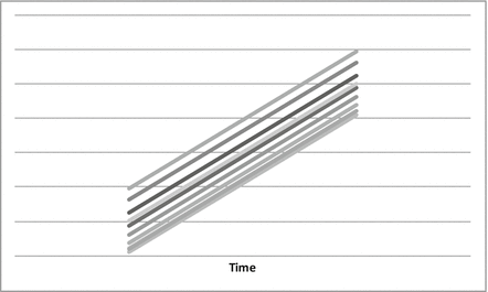
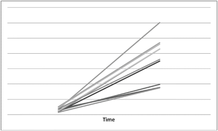
The idea behind MM (Twisk 2013) was initially developed in the social sciences, specifically for educational research. Investigating the performance of pupils within schools, researchers realised that the performances of pupils within the same class were not independent (in other words; these performances are correlated). This type of study design is characterised by a hierarchical structure; also referred to as a multilevel structure. Pupils are nested within classes and classes are nested within schools. More or less the same structure is seen in longitudinal datasets where observations are nested within the subject: observations of one subject over time are correlated. MM adjusts for this correlation between repeated observations by modelling the variability among individuals through the inclusion of both fixed and random effects. To understand the general idea behind a mixed model, it is important to realise that with simple regression analyses adjusting for a certain variable (for example gender) means that different intercepts are calculated. In a longitudinal setting (thus adjusting for subject), this then means that for each subject, different intercepts are calculated. The simplest form of a MM takes into account this random intercept only. Figure 9.1 demonstrates that a model with a random intercept only allows the intercepts to vary across subjects. In addition to a random intercept, it is also possible that the development over time varies across individuals (indicated by a random slope). This is demonstrated in Fig. 9.2, where only linear slopes are assumed.

Within life course epidemiology, MM are usually conducted to describe the development of a particular outcome variable over time (Beunen et al. 2002; Twisk 2013). In that case, the only independent variable of interest is a time variable, which can be included either as a continuous variable (indicating a linear development or other polynomial function of the outcome variable over time) or as a categorical variable. The modelling of time as a categorical variable allows for the incorporation of different developmental shapes during different stages in the life course, such as childhood, adolescence, adulthood and the elderly. This closely maps onto one of the focal points of life course research, which offers opportunities to understand the natural history of chronic disorders with a specific focus on health transitions and phases across the life course (Kuh and Ben-Shlomo 2004).

Model fit of MM can be assessed by comparing the log likelihood values of neighbouring [nested] models. The likelihood ratio test (Bollen 1989) subsequently calculates the difference in -2 log-likelihood between two neighbouring models. This difference is assumed to follow a Chi-squared distribution with the number of degrees of freedom denoted as the difference in the number of parameters estimated with the two models.

The simplest model includes a random intercept only. Table 9.2 demonstrates the results of this model and indicates that body mass index values are increasing over time. The regression coefficient for time for the linear model (model 1) is 0.240, so for each year, the BMI increases (linearly) with 0.240 kg/m². The corresponding standard error (0.003; indicative of the preciseness in the estimation of the regression coefficient – the smaller the more precise) can be used to assess the statistical significance of the regression coefficient by calculating the z-statistic (Altman 1991; Twisk 2013). The z-statistic is calculated by dividing the regression coefficient with the corresponding standard error. Values above 1.96 indicate statistical significance.