where j ≠ k, j = 1, …, 4, k = 1, …, 4.
The infected region or ROI cannot be easily represented by standard measurement of length, area, shape, and size causing the selection of feature vectors difficult for any discrimination procedure. Henceforth, any standard image processing technique such as image enhancement or segmentation is avoided as much as possible to avoid possible lost of information from the original image.
4.2 Materials and Methods
4.2.1 Selection of Case Study
This study involved collaboration with the Institute of Respiratory Medicine (IPR), Malaysia, which is the national referral center for respiratory diseases. Cases that arrived at the IPR may be considered a random sample since an individual case may come from any of the Malaysian hospitals or clinics. The IPR provided archived patients’ data which include chest X-ray films captured using the Phillips Diagnost 55/Super 50CP (Phillips Corp., Holland) together with complete patients’ medical information. The patients’ chest were captured in full inspiration using the posterior–anterior (PA) view with distance from the X-ray to the patient is fixed at 180 cm to diminish the effect of beam divergence and magnification of structures closer to the X-ray tube. The cassette size of 35 × 35 cm is used for female chest and 35 × 34 cm for male chest. The patient is exposed to 64 kV and 4.0 mAs if underweight, and 70 kV and 5.0 mAs if the patient has normal weight.
The archived data (stored in files) in IPR were diagnosed by a pulmonologist. In IPR, all the pulmonologists are trained to interpret chest radiographs. Stratified random sampling (SRS) was carried out for the patients’ file. SRS means that files were randomly selected given that the patients chosen were already diagnosed as PTB or LC. The role of the consultant pulmonologist is to verify the diagnosis. It should be noted that the pulmonologist and consultant pulmonologist mentioned above are two different individuals.
The patient’s chest X-ray is then divided into two groups, which are the control group and the test group. The selected patients used as the control group were the confirmed pneumonia (PNEU), pulmonary tuberculosis (PTB), and lung cancer (LC) cases with no other systemic diseases such as diabetes, hypertension, and heart disease. The omission of cases with other systemic diseases was done in order to avoid bias in the development of the statistical discriminant function (DF). The test group was selected similarly except that some of the patients may have other systemic diseases.
Lobar pneumonia is defined when one section or lobe of the lung is affected. In diagnosing pneumonia, the patient is assessed for crackles and wheezing sound from the lung, using a stethoscope (Wipf et al. 1999). The radiographic interpretation is considered the gold standard for the presence of pneumonia where the physical findings is accurate if it is found in the same location as an infiltrate on chest X-ray (Wipf et al. 1999). The confirmation of the PTB cases is based on the clinical feature (symptoms and sign), chest X-ray examination, and sputum Acid Fast Bacilli (AFB) direct smear. For the lung cancer, cases under study consist of 75 % cases of non-small cell carcinoma (of which 50 % are the squamous cell carcinoma and 25 % are the adenocarcinoma) and 25 % cases of small cell carcinoma. The confirmation of LC was based on bronchial biopsy result. The normal lung (NL) chest X-ray films selected by the radiologist from Universiti Sains Malaysia Hospital (HUSM) represent patients who came for a general medical checkup.
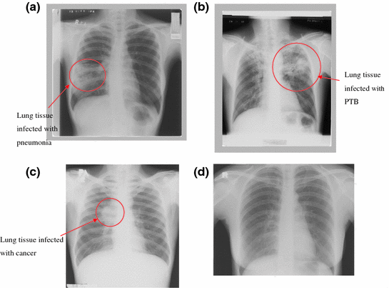
Patients that have lung disease (either PNEU, PTB, or LC) will have their chest X-ray film image shows some abnormal opacity. The existence of lung consolidation in the chest X-ray may confirm the existence of pneumonia and may appear on the chest X-ray after a few days of infection. The PTB image will show multiple opacities of varying size that run together (coalesce) in the chest X-ray image. Severe cases of PTB may result in consolidation and cavity, and the scarring marks may remain visible in the chest X-ray even after the patient is cured. Lung cancer appears as a mass opacity in the chest X-ray image. The chest radiograph image of a normal lung will show a complete dark image between rib bones due to nonexistence of any hardened substances.
The chest X-ray films were then digitized into DICOM format using the Kodak LS 75 X-ray Film Scanner (pixel spot size of 100 μm, 12 bit per pixel, image size of 2016 × 2048 pixels). An example of a digitized X-ray film is shown in Fig. 4.1a–d.


Fig. 4.1
a Visual of chest radiograph of pneumonia-infected lung (source The Institute of Respiratory Medicine, Kuala Lumpur). b Example of chest radiograph showing PTB-infected lung (snowflakes) (source The Institute of Respiratory Medicine, Kuala Lumpur). c Example of chest radiograph showing lung cancer (source The Institute of Respiratory Medicine, Kuala Lumpur). d Example of normal lung of an healthy individual (source The Institute of Respiratory Medicine, Kuala Lumpur)
4.2.2 Texture Measures
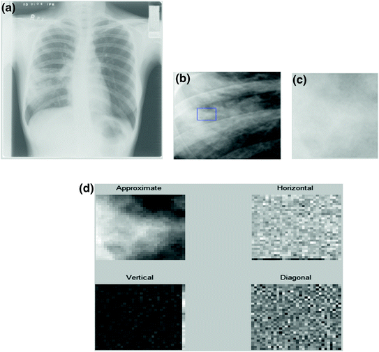
Each of the ROI for a given image was subjected to the two-dimensional Daubechies wavelet transform as shown in Fig. 4.2, (Daubechies 1992; Walker 1999). The wavelet transform convert the image into four subsets, labeled LL, LH, HL, and HH representing the trend, horizontal, vertical, and diagonal detail coefficients.


Fig. 4.2
a Chest X-ray of a pneumonia patient and b a subset image of the infected area. c Region of interest and d the transformed image where four image subset was formed (source The Institute of Respiratory Medicine, Kuala Lumpur)
The twelve texture measures considered were as follows:
1.
Mean Energy, 

2.


3.
Contrast = 

4.
Homogeneity, 

5.
Standard deviation of value,  where
where 
 where
where 
6.
Standard deviation of energy,  where
where 
 where
where 
7.
Maximum wavelet coefficient value, max = max(C jk )
8.
Minimum wavelet coefficient value, min = min(C jk )
9.
Maximum value of energy, 

10.
Maximum row sum energy
11.
Maximum column sum energy
12.
Average number of zero-crossings
4.2.3 Modified Principal Component Method
The modified principal component (ModPC) method was introduced in (Noor et al. 2010) where PNEU is discriminated from normals. The ModPC method is now extended for pair-wise comparison between three types of diseases namely, PNEU, PTB, LC, and normals.
A sample of 200 images were concurrently read and interpreted for the presence of PNEU, PTB, LC, and normals by two independent pulmonologists who are trained according to the World Health Organization (WHO) guideline (WHO Report 2004; Cherian et al. 2005), and the affected region (ROI) was identified.
The data used were divided into two sets, ( ) as the control data set and (
 ) as the test data set. Let,
 ) as the control data set and (
 ) as the test data set. Let,
 represents the texture measures for PNEU samples,
 represents the texture measures for normal lung samples,
 represents the texture measures for PTB samples, and
  represents the texture measures for LC samples.
The main problem of the ModPC method is the choice of an orthogonal transformation. Let M be an orthogonal matrix such that


Let  be the estimate of the covariance matrix for group G j (j = 1, …, 4). For example,
 while S 2, S 3, and S 4 were similarly defined for the sets G 2, G 3, and G 4, respectively.
 be the estimate of the covariance matrix for group G j (j = 1, …, 4). For example,
The spectral decomposition of the estimated covariance matrices are
 where n = 30, Q j (j = 1, …, 4) is the appropriate matrix of eigenvectors, and Λ j (j = 1,…, 4) is the corresponding diagonal matrix of eigenvalues. Henceforth, the choice of M will depend on minimizing misclassification probabilities in a two population discrimination problems. In particular, choose M = Q j or M = Q k (j ≠ k), j = 1, …, 4 and k = 1, …, 4 such that the probability of misclassifying the test data to either population-j or population-k is minimized.

Without loss of generality, consider the two population discrimination problems PNEU and NL. For a selected M matrix, take the first two components of  , which explain at least 90 % of the variability, relabel it as v r (r = 1, …, 30), and perform the following:
 , which explain at least 90 % of the variability, relabel it as v r (r = 1, …, 30), and perform the following:
For vectors,  calculate the statistics
  and
and  . The vectors v 1, v 2, …, v 30 were found to be bivariate normal (see Sect. 4.2.4). Henceforth, the PNEU ellipsoid
  was drawn where c was selected from a standard Chi square table (see Sect. 4.2.5). Further, the estimate of g 1(v), which is the probability distribution for G 1 was also obtained.
 calculate the statistics
  and
and  . The vectors v 1, v 2, …, v 30 were found to be bivariate normal (see Sect. 4.2.4). Henceforth, the PNEU ellipsoid
  was drawn where c was selected from a standard Chi square table (see Sect. 4.2.5). Further, the estimate of g 1(v), which is the probability distribution for G 1 was also obtained.
The above was repeated for v 31, v 32, …, v 60 yielding, say the NL ellipsoid and the corresponding estimate of g 2(v) which is the probability distribution for G 2. Finally, the estimate of the discriminant function  may be derived (Johnson and Wichern 2007). Two-dimensional probability ellipsoids and appropriate DFs estimate the following error probability;

and

for a selected texture measure.
 may be derived (Johnson and Wichern 2007). Two-dimensional probability ellipsoids and appropriate DFs estimate the following error probability;
(4.1)

(4.2)
For the PNEU–NL discrimination problem, there are two ways of estimating the error probabilities α and β by using the test set v 121, v 62, …, v 140 from G 1 and v 141, v 82, …, v 160 from G 2 in two ways where  are the first two components of
  ;
;
 are the first two components of
  ;
;(a)
Estimation of α and β from the probability ellipsoid:
1.
The number of times  falls into the NL ellipsoid gives an estimate of β.
 falls into the NL ellipsoid gives an estimate of β.
2.
The number of times  falls into the PNEU ellipsoid gives an estimate of α.
 falls into the PNEU ellipsoid gives an estimate of α.
(b)
Estimation of α and β from DF:
Investigate if 

where g 1(v), the probability distribution for PNEU, was found to be  and g 2(v), the probability distribution for NL was shown to be
  . Further,
  where d(i|j) is the cost of misclassifying observation-j (i = 1, 2 and j = 1, 2), while p 1 and p 2 are the a priori probabilities. Suppose v * is an unknown observation and assuming that p 1 = p 2 and d(1|2) = d(2|1), then v * is assigned to the PNEU group if DF12(v *) > 0, otherwise it is assigned to the NL group.
 and g 2(v), the probability distribution for NL was shown to be
  . Further,
  where d(i|j) is the cost of misclassifying observation-j (i = 1, 2 and j = 1, 2), while p 1 and p 2 are the a priori probabilities. Suppose v * is an unknown observation and assuming that p 1 = p 2 and d(1|2) = d(2|1), then v * is assigned to the PNEU group if DF12(v *) > 0, otherwise it is assigned to the NL group.
The equality of covariance matrices was tested using the Box’s Test (Mardia et al. 1979), and if  , DF12(v) is the linear discriminant function (LDF), which allocates the unknown observation m 0 as follows;
 , DF12(v) is the linear discriminant function (LDF), which allocates the unknown observation m 0 as follows;
Allocate m 0 to population one if
![$$ \left[ {(\underline{\mu }_{1} - \underline{\mu }_{2} )^{T} \varSigma^{ - 1} (\underline{m}_{0} ) + \frac{1}{2}(\underline{\mu }_{1} - \underline{\mu }_{2} )^{T} \varSigma^{ - 1} (\underline{\mu }_{1} + \underline{\mu }_{2} )} \right] \ge \ln \left[ {\left( {\frac{d(1|2)}{d(2|1)}} \right)\left( {\frac{{p_{2} }}{{p_{1} }}} \right)} \right] $$](/wp-content/uploads/2017/03/A313638_1_En_4_Chapter_Equ3.gif)
![$$ \left[ {(\underline{\mu }_{1} - \underline{\mu }_{2} )^{T} \varSigma^{ - 1} (\underline{m}_{0} ) + \frac{1}{2}(\underline{\mu }_{1} - \underline{\mu }_{2} )^{T} \varSigma^{ - 1} (\underline{\mu }_{1} + \underline{\mu }_{2} )} \right] \ge \ln \left[ {\left( {\frac{d(1|2)}{d(2|1)}} \right)\left( {\frac{{p_{2} }}{{p_{1} }}} \right)} \right] $$](/wp-content/uploads/2017/03/A313638_1_En_4_Chapter_Equ3.gif)
(4.3)
Otherwise allocate m 0 to population two.
Alternatively, if  then DF12(v) is the quadratic discriminant function (QDF), which allocates the unknown m 0 as follows;
 then DF12(v) is the quadratic discriminant function (QDF), which allocates the unknown m 0 as follows;
Allocate m 0 to population one if
![$$ \left[ { - \frac{1}{2}\underline{m}_{0}^{T} \varSigma_{1}^{ - 1} - \varSigma_{2}^{ - 1} \underline{m}_{0} + (\underline{\mu }_{1}^{T} \varSigma_{1}^{ - 1} - \underline{\mu }_{2}^{T} \varSigma_{2}^{ - 1} )^{T} \underline{m}_{0} - k} \right] \ge \left( {\frac{d(1|2)}{d(2|1)}} \right)\left( {\frac{{p_{2} }}{{p_{1} }}} \right) $$](/wp-content/uploads/2017/03/A313638_1_En_4_Chapter_Equ4.gif)
where  .
.
![$$ \left[ { - \frac{1}{2}\underline{m}_{0}^{T} \varSigma_{1}^{ - 1} - \varSigma_{2}^{ - 1} \underline{m}_{0} + (\underline{\mu }_{1}^{T} \varSigma_{1}^{ - 1} - \underline{\mu }_{2}^{T} \varSigma_{2}^{ - 1} )^{T} \underline{m}_{0} - k} \right] \ge \left( {\frac{d(1|2)}{d(2|1)}} \right)\left( {\frac{{p_{2} }}{{p_{1} }}} \right) $$](/wp-content/uploads/2017/03/A313638_1_En_4_Chapter_Equ4.gif)
(4.4)
 .
.Otherwise allocate m 0 to population two.
Throughout the study it is assumed that d(1|2) = d(2|1) and p 1 = p 2 for both Eqs. 4.3 and 4.4. These assumptions were taken because the event of having either disease is regarded with having equal weight, and equal a prior probability is because there is no true or exact information about total frequency of cases in Malaysia.
Henceforth, the number of times DF12(v j ) < 0 for  gives an estimate of β. Likewise, α is similarly derived.
 gives an estimate of β. Likewise, α is similarly derived.
All the above were repeated for the second selection of M (say M = Q k ) and suppose this choice yields lower α and β values, then M = Q k will be the preferred choice. Tables 4.1 and 4.2 illustrate all the combination of the two population discrimination problem studied. Flowchart shown in Fig. 4.3 illustrates the discrimination problem for the disease present and disease absent cases. Flowchart shown in Fig. 4.4 gives similar illustration for the pair-wise comparison of diseases.
Table 4.1


Pair-wise discrimination strategy between disease absent (DA) and disease present (DP)
Stay updated, free articles. Join our Telegram channel

Full access? Get Clinical Tree


