Maia Martcheva1
(1)
Department of Mathematics, University of Florida, Gainesville, FL, USA
5.1 Building Complex Epidemiological Models
In the previous chapters, we introduced and studied the simplest epidemic models: the SIR model, the SIS model, and the Ross–MacDonald model of vector-borne disease. The baseline SI, SIS, SIR, and SIRS epidemic models can be extended to incorporate more realistic features of the disease, various control strategies, and heterogeneities of the host and the pathogens. As the models become more complex, their flowcharts also become more complex, with more compartments and transitions. Developing a flowchart of a complex model that is both clear and informative is more of an art than a science. Furthermore, as more realistic features are incorporated in the models and the systems become higher-dimensional, we need better tools for the computation of the reproduction number  . In this chapter, we build models with more realism and introduce techniques for the computation of the reproduction number.
 . In this chapter, we build models with more realism and introduce techniques for the computation of the reproduction number.
The baseline SI, SIS, and SIR models are developed based on essential components of the infectious disease transmission process: the presence of susceptible and infectious individuals. However, for many diseases, the natural progression of the disease may contain various other components that affect the disease transmission, and ultimately the conclusions we will make from the model.
5.1.1 Stages Related to Disease Progression
The most important stages of the disease other than susceptible and infectious that affect transmission are the (1) exposed/latent stage; (2) asymptomatic stage; (3) carrier stage; (4) passive immunity stage.
1.
Exposed/Latent Stage. For many diseases, the infected individuals do not become immediately infectious, as assumed in the SIS and SIR models. The pathogen needs time to replicate and establish itself in the new host. The time during which an individual is infected but not yet infectious is called the latent period. As an additional compartment in epidemiological models, the latent period is denoted by E(t) or by L(t). We note that the incubation period of a pathogen is the period between infection and onset of symptoms. The lengths of the latent and incubation periods do not necessarily coincide. For instance, in influenza, the onset of symptoms begins one day after infected individuals have become infectious; that is, the incubation period is one day longer than the latent period. The exposed (latent) period usually follows the susceptible stage. If we introduce a latent period in the SI model, the resulting model is an SEI model; if we introduce a latent period in the SIR model, the resulting model is an SEIR model. Similarly, we can have SEIS and SEIRS models based respectively on SIS and SIRS models. The SEIR model takes the form
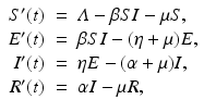
where η is the per capita rate of becoming infectious. We recall that 1∕η is approximately the length of the latent period. The flowchart of the SEIR model is given in Fig. 5.1.


(5.1)

Fig. 5.1
Flowchart of the SEIR model. Demographic rates are not included
2.
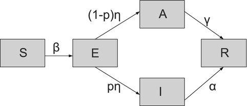
Asymptomatic Stage. The asymptomatic compartment is usually included to incorporate asymptomatic infection. Asymptomatic infection, also often called subclinical infection, is an infection without symptoms. Individuals with asymptomatic infection are still infectious and contribute to the distribution of the disease. However, because they do not show symptoms, they are much harder to detect. Asymptomatic infection has been shown to exist for many diseases, including HIV, malaria, dengue, measles, polio, and influenza. An asymptomatic compartment is typically included as an alternative to the infectious compartment I. The asymptomatic compartment is denoted by A(t). Exposed individuals progress to the symptomatic infectious compartment with probability p, and to the asymptomatic infectious compartment with probability (1 − p). Asymptomatic individuals are typically assumed to be infectious at a reduced transmission rate q β:
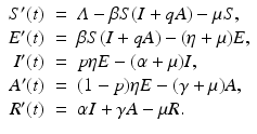
The parameter γ gives the recovery rate of the asymptomatic individuals. Often, the symptomatic infectious period is longer than the asymptomatic:  . A flowchart of the model with asymptomatic infection is shown in Fig. 5.2.

(5.2)
 . A flowchart of the model with asymptomatic infection is shown in Fig. 5.2.
Fig. 5.2
Flowchart of the SEIR model with asymptomatic stage model. Demographic rates are not included
3.
Carrier Stage. A carrier stage is incorporated to account for individuals who are otherwise healthy but harbor and transmit the pathogen. Carriers show no symptoms or signs of infection, but the disease microorganisms can be recovered from their nose, throat, or feces. Carrier individuals contribute to the distribution of the disease without being sick themselves. Alternatively, a pathogen carrier may be someone who has been infected and was not treated because the infection was asymptomatic, or was incompletely treated. Several viral and bacterial diseases exhibit a carrier stage. Viral diseases, such as viral hepatitis and poliomyelitis, and bacterial diseases, including diphtheria and meningococcal meningitis, often have a carrier stage. The carrier compartment is usually denoted by C(t). An SIRS model with carrier stage is included below:
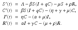
Individuals are assumed to enter the carrier stage upon infection. Then some progress to being infected and infectious, while others recover from the pathogen without ever being infected. A flowchart of the model is given in Fig. 5.3.
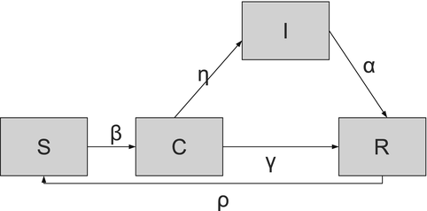

(5.3)

Fig. 5.3
Flowchart of the SCIRS model. Demographic rates are not included
4.
Passive Immunity Stage. Passive immunity is the transfer of active immunity in the form of antibodies from one individual to another. Passive immunity can occur naturally, when maternal antibodies are transferred to the fetus through the placenta or in the milk during breastfeeding. Passive immunity can also be induced artificially, when high levels of antibodies specific for a pathogen or toxin are transferred to nonimmune individuals. Mathematical models typically involve natural passive immunity. The passive immunity stage is often denoted by M(t), and it is added to the system before individuals become susceptible. An MSIR model with passive immunity has the form
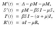
where ρ is the per unit of time rate of loss of maternal antibodies. We assume that babies are completely protected by the maternal antibodies and cannot get infected.

(5.4)
5.1.2 Stages Related to Control Strategies
Besides involving compartments related to the various disease-progression stages, basic baseline SI, SIS, SIR, and SIRS models may involve compartments associated with the various strategies applied for control of the disease. Disease-control strategies involve (1) quarantine/isolation; (2) vaccination; (3) treatment.
1.
Quarantine/isolation. Quarantine is compulsory isolation, typically to contain the spread of a disease. The word comes from the Italian (seventeenth-century Venetian) quarantena, meaning a 40-day period. Quarantine is applied to individuals who have come into contact with an infectious individual and may or may not be infected. Isolation is confinement of an infectious individual that restricts that individual’s contact with healthy susceptible individuals. Isolation is applied to infectious individuals only. The class of quarantines/isolated individuals is typically denoted by Q(t). An SIQR model is given below. Standard, rather than mass-action, incidence is assumed [61]. We note that the “total” population size consists of all individuals that participate in the mixing. We call all individuals that participate in the mixing active individuals, and denote the size of the active class by  :
:
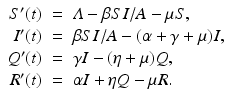
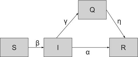
SIQR models are appropriate to model childhood diseases. Quarantine has been found to destabilize the epidemic and lead to sustained oscillations in the dynamics of childhood diseases [61]. A flowchart of the SIQR model is given in Fig. 5.4.
 :
:
(5.5)

Fig. 5.4
Flowchart of the SIQR model. Demographic rates are not included
2.
Treatment. Treatment is the care provided to reduce morbidity and mortality of an infectious disease. Treatment usually includes administering medication that mitigates symptoms and helps the immune system fight the pathogen. A treatment compartment T(t) has been included in standard SEI epidemic models as a class that replaces the class of recovered individuals, making the model an SEIT model. Since patients often do not complete the full regimen of treatment, treatment may or may not be successful, and leads to the individual being successfully treated with probability q or relapsing to the exposed/latent class with probability p, where  . The model with treatment is presented below, and it captures the dynamics of a disease such as tuberculosis [60]:

where r 1 is the treatment rate of exposed individuals, r 2 is the treatment rate of infectious individuals, and κ is the progression to the infectious state. The presence of relapsing individuals leads to ambiguity in the computation of the reproduction number, which we will discuss later. A flowchart of the model is given in Fig. 5.5.
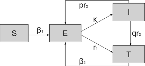
 . The model with treatment is presented below, and it captures the dynamics of a disease such as tuberculosis [60]:
(5.6)

Fig. 5.5
Flowchart of the SEIT model. Demographic rates are not included
3.
Vaccination. Vaccination is the administration of generally dead or weakened antigenic material (a vaccine) to produce immunity to a disease. There are two main ways to incorporate vaccination in an epidemic model. In the first approach vaccine is administered to individuals who are entering the system. A proportion p of entering individuals enters the susceptible class, while a proportion 1 − p enters the recovered/immune class. In the second approach, susceptible individuals are continuously being vaccinated and move to the vaccinated class V (t). Vaccination may provide complete or partial immunity to the disease. We will consider vaccination in more detail in Chap. 9
5.1.3 Stages Related to Pathogen or Host Heterogeneity
The impact of host or pathogen heterogeneities on the dynamics of the disease has been a longstanding question of interest in mathematical epidemiology. We will consider the following heterogeneities:
1.
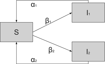
Pathogen Genetic Heterogeneities. Many pathogens are represented by multiple genetically distinct variants. The presence of the variants has implication for the disease progression and control as different pathogen variants respond differently to the control measures. To study pathogen heterogeneities, two-strain and multistrain models have been developed. The simplest SIS model with two strains includes the number of infected with strain one I 1 and the number of infected with strain two I 2:

We address the interplay between pathogen heterogeneity and disease transmission dynamics in Chap. 8 A flowchart of the two-strain model above is given in Fig. 5.6.

(5.7)

Fig. 5.6
Flowchart of the two-strain model. Demographic rates are not included
2.
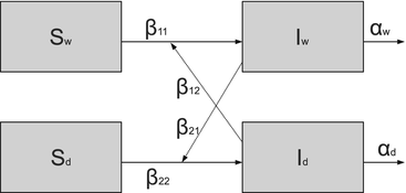
Host Heterogeneities. Host heterogeneities in susceptibility and infectivity associated with host genetic differences can lead to models with multiple host species. For instance, in avian influenza, the pathogen can infect both wild birds and domestic birds. These two categories of birds can have very different demographic characteristics as well as different characteristics with respect to the disease. To account for the differences, a simple SI model should have two susceptible populations S w and S d and two infected populations I w and I d . The multihost single-pathogen model takes the form

A flowchart of the model is given in Fig. 5.7.

(5.8)

Fig. 5.7
Flowchart of the two-strain model. Demographic rates are not included
3.
Age and Space Heterogeneities. Age and space heterogeneities are introduced respectively by the age of the host and the presence of a spatial component in the transmission of the disease. Age and space heterogeneities can be incorporated in the model as a continuous component, which results in partial differential equations, or as a discrete component, which results in larger systems of ordinary differential equations. These heterogeneities will be discussed in Chaps. 16 and 15.
5.2 Jacobian Approach for the Computation of 
We saw in the previous chapters that mathematically, the reproduction number  gives a threshold condition for the stability of the disease-free equilibrium. Imposing conditions for stability leads to an expression for the reproduction number. This general approach can also be applied in more complex models. In particular, we compute the Jacobian of the system at the disease-free equilibrium, and we pose the condition that all eigenvalues of the corresponding characteristic equation must have negative real parts. In the two-dimensional case, this requirement follows from the conditions that TrJ < 0 and DetJ > 0. In the higher-dimensional case, this theorem does not apply, but one can often reduce the characteristic equation to the two-dimensional case using the properties for manipulation of matrices. Even when we have a unique condition for the stability of the disease-free equilibrium, rewriting this condition in the form of a reproduction number can often be done in more than one way. It is typically expected that the expression for the reproduction number should satisfy the following conditions.
 gives a threshold condition for the stability of the disease-free equilibrium. Imposing conditions for stability leads to an expression for the reproduction number. This general approach can also be applied in more complex models. In particular, we compute the Jacobian of the system at the disease-free equilibrium, and we pose the condition that all eigenvalues of the corresponding characteristic equation must have negative real parts. In the two-dimensional case, this requirement follows from the conditions that TrJ < 0 and DetJ > 0. In the higher-dimensional case, this theorem does not apply, but one can often reduce the characteristic equation to the two-dimensional case using the properties for manipulation of matrices. Even when we have a unique condition for the stability of the disease-free equilibrium, rewriting this condition in the form of a reproduction number can often be done in more than one way. It is typically expected that the expression for the reproduction number should satisfy the following conditions.
The reproduction number should:
Be nonnegative for nonnegative parameter values;
Be zero if there is no transmission;
Be interpretable as the number of secondary infections.
5.2.1 Examples in Which the Jacobian Reduces to a 2 × 2 Matrix
As a first higher-dimensional example, we consider the SIRS model with carrier stage (5.3). The disease-free equilibrium for that model is given as  , where the variables are arranged in the same way as the equations in the system. Computing the Jacobian at the disease-free equilibrium gives

where  . If we consider
  , we can expand the matrix in terms of the first column. This will give an eigenvalue
  . Then we can expand the remaining matrix around the last column. This will give an eigenvalue
  . The remaining two eigenvalues are the eigenvalues of the following matrix:

Now we can apply the usual conditions that guarantee that the eigenvalues of J 1 have negative real part. In particular, we want Tr J 1 < 0 and Det J 1 > 0. The second inequality gives  -\eta \beta S^{{\ast}} > 0$$
” src=”/wp-content/uploads/2016/11/A304573_1_En_5_Chapter_IEq12.gif”></SPAN>. This condition gives a reproduction number in the form<br />
<DIV id=Equa class=Equation><br />
<DIV class=EquationContent><br />
<DIV class=MediaObject><IMG alt=](/wp-content/uploads/2016/11/A304573_1_En_5_Chapter_Equa.gif)
 , where the variables are arranged in the same way as the equations in the system. Computing the Jacobian at the disease-free equilibrium gives
(5.9)
 . If we consider
  , we can expand the matrix in terms of the first column. This will give an eigenvalue
  . Then we can expand the remaining matrix around the last column. This will give an eigenvalue
  . The remaining two eigenvalues are the eigenvalues of the following matrix:
(5.10)
 -\eta \beta S^{{\ast}} > 0$$
” src=”/wp-content/uploads/2016/11/A304573_1_En_5_Chapter_IEq12.gif”></SPAN>. This condition gives a reproduction number in the form<br />
<DIV id=Equa class=Equation><br />
<DIV class=EquationContent><br />
<DIV class=MediaObject><IMG alt=](/wp-content/uploads/2016/11/A304573_1_En_5_Chapter_Equa.gif)
 implies both Tr J 1 < 0 and Det J 1 > 0. Therefore, if
  , the disease-free equilibrium is locally asymptotically stable. If
  . Hence, the first term gives the number of secondary infections produced by a carrier in an entirely susceptible population during its lifetime as a carrier. Similarly, β S I is the incidence of an infected individual. Hence, the number of secondary infections that one infectious individual will produce in an entirely susceptible population per unit of time is β S ∗. The number of time units spent in the carrier compartment is
  . The newly infected individual becomes a carrier, and the fraction of carriers that survive the carrier stage and become infected is
  . We see that the second term gives the number of secondary infections produced by an infectious individual in an entirely susceptible population during its lifetime as infectious.
5.2.2 Routh–Hurwitz Criteria in Higher Dimensions
For many higher-dimensional models, the Jacobian computed at the disease-free equilibrium cannot be reduced to a 2 × 2 matrix. The characteristic polynomial then has degree three or higher. In this case, the reproduction number can be obtained from the constant term. Whether the reproduction number is greater or less than 1 determines the sign of the constant term. Nonetheless, we still need tools that give necessary and sufficient conditions for the eigenvalues to have negative real parts. These conditions are given by the Routh–Hurwitz criterion, which is stated in the following theorem:
Theorem 5.1 (Routh–Hurwitz Criteria).
Consider the nth-degree polynomial with real constant coefficients
 Define n Hurwitz matrices using the coefficients a i of the characteristic polynomial:
 and
and
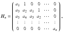 where a j = 0 if j > n. All roots of the polynomial P(λ) are negative or have negative real part if and only if the determinants of all Hurwitz matrices are positive:
![$$\displaystyle{\mathrm{Det}\,H_{j} > 0,\qquad j = 1,\ldots,n.}$$
” src=”/wp-content/uploads/2016/11/A304573_1_En_5_Chapter_Eque.gif”></DIV></DIV></DIV></DIV></DIV><br />
<DIV class=Para>For <SPAN class=EmphasisTypeItalic>n</SPAN> = 2, the Routh–Hurwitz criterion simplifies to <SPAN class=EmphasisTypeItalic>a</SPAN> <SUB>1</SUB> > 0 and <SPAN class=EmphasisTypeItalic>a</SPAN> <SUB>1</SUB> <SPAN class=EmphasisTypeItalic>a</SPAN> <SUB>2</SUB> > 0. We note that <SPAN class=EmphasisTypeItalic>a</SPAN> <SUB>3</SUB> = 0 in <SPAN class=EmphasisTypeItalic>H</SPAN> <SUB>2</SUB>. These conditions are equivalent to <SPAN class=EmphasisTypeItalic>a</SPAN> <SUB>1</SUB> > 0 and <SPAN class=EmphasisTypeItalic>a</SPAN> <SUB>2</SUB> > 0 and are analogous to the conditions we applied before: Tr <SPAN class=EmphasisTypeItalic>J</SPAN> < 0 and Det <SPAN class=EmphasisTypeItalic>J</SPAN> > 0. The Routh–Hurwitz criteria for polynomials are given in Table <SPAN class=InternalRef><A href=]() 5.1. A necessary but not sufficient condition for the roots of the polynomial P(λ) to be negative or have negative real part is that all coefficients be strictly positive. This is required in the column labeled Coefficient signs in Table 5.1.
5.1. A necessary but not sufficient condition for the roots of the polynomial P(λ) to be negative or have negative real part is that all coefficients be strictly positive. This is required in the column labeled Coefficient signs in Table 5.1.


Table 5.1
Routh–Hurwitz criteria
n | Coefficient signs | Additional conditions |
|---|---|---|
2 | a 1 > 0, a 2 > 0 | – |
3 | a 1 > 0, a 2 > 0, a 3 > 0 | a 1 a 2 > a 3 |
4 | a 1 > 0, a 2 > 0, a 3 > 0, a 4 > 0 | a 1 a 2 a 3 > a 3 2 + a 1 2 a 4 |
5 | a 1 > 0, a 2 > 0, a 3 > 0, a 4 > 0, | a 1 a 2 a 3 > a 3 2 + a 1 2 a 4, |
a 5 > 0 |  , where , where  . The Jacobian at the disease-free equilibrium is . The Jacobian at the disease-free equilibrium is (5.11)  by the first column and then by the last column, we obtain two of the eigenvalues of J: by the first column and then by the last column, we obtain two of the eigenvalues of J:  and and  . The remaining three eigenvalues are the eigenvalues of the 3 × 3 matrix . The remaining three eigenvalues are the eigenvalues of the 3 × 3 matrix (5.12)   (5.13)    should be equivalent to the condition a 3 > 0. Hence, we define should be equivalent to the condition a 3 > 0. Hence, we define  as follows: as follows:  . Furthermore, if . Furthermore, if  , the equation P(λ) = 0 has a real positive solution, and the disease-free equilibrium is therefore unstable. It remains to see that if , the equation P(λ) = 0 has a real positive solution, and the disease-free equilibrium is therefore unstable. It remains to see that if  , the disease-free equilibrium is locally asymptotically stable. In particular, we have to show that in this case, the equation P(λ) = 0 has only negative roots or roots with negative real part. To see this, we use the Routh–Hurwitz criteria for dimension three. The Routh–Hurwitz conditions for stability for dimension three are listed in Table 5.1. We see that from the condition , the disease-free equilibrium is locally asymptotically stable. In particular, we have to show that in this case, the equation P(λ) = 0 has only negative roots or roots with negative real part. To see this, we use the Routh–Hurwitz criteria for dimension three. The Routh–Hurwitz conditions for stability for dimension three are listed in Table 5.1. We see that from the condition  , it follows that a 3 > 0. Clearly a 1 > 0. The condition , it follows that a 3 > 0. Clearly a 1 > 0. The condition  also gives also gives  . Consequently, . Consequently, . Mathematically, the above definition of . Mathematically, the above definition of  is sound. To be sound epidemiologically, the reproduction number should be interpretable as the number of secondary cases. To see this, first notice that the reproduction number is a sum of two terms. The first term gives the number of secondary infections of asymptomatic individuals produced by one asymptomatic individual. Indeed, q β S ∗ is the number of newly exposed individuals generated by one asymptomatic individual per unit of time in an entirely susceptible population. A fraction is sound. To be sound epidemiologically, the reproduction number should be interpretable as the number of secondary cases. To see this, first notice that the reproduction number is a sum of two terms. The first term gives the number of secondary infections of asymptomatic individuals produced by one asymptomatic individual. Indeed, q β S ∗ is the number of newly exposed individuals generated by one asymptomatic individual per unit of time in an entirely susceptible population. A fraction  survives the exposed stage and progresses to the asymptomatic stage. One asymptomatic individual remains asymptomatic and infects other individuals as asymptomatic for survives the exposed stage and progresses to the asymptomatic stage. One asymptomatic individual remains asymptomatic and infects other individuals as asymptomatic for  units. Hence, units. Hence,  survives the exposed stage and progresses to the infectious stage. One infectious individual remains infectious to susceptible individuals for survives the exposed stage and progresses to the infectious stage. One infectious individual remains infectious to susceptible individuals for  units. Hence, units. Hence,
|


