Estimating a population statistic

Research studies are carried out to answer specific questions about the health of a group of people, for example:

In the first case, we say that the target population, i.e. the population of interest, is all men aged over 65 in the UK. This can be expanded to include all future men aged > 65 in the UK. However, we clearly can’t find all these men, and measure their systolic blood pressures and ask about whether they smoke. Instead, we use a study sample to make inferences about the target population (see Figure 4.1).

Figure 4.1 Using statistical methods to make inferences about the population, in a research study.

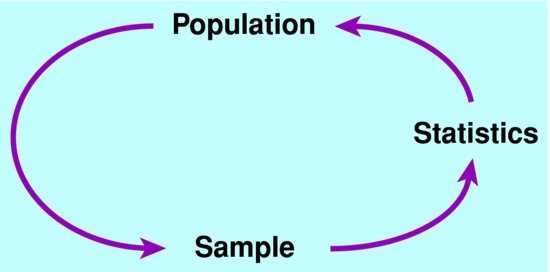
There are two ways in which a sample can be considered representative of a target population. The first is where we have a list of the people in the target population (e.g. all men in the UK aged > 65, from census or General Practice records) and we randomly select the study sample from this (e.g. randomly select a number of men aged > 65 from census records). The second is to use eligibility criteria for the study sample, and then assume that the study sample represents all people satisfying those criteria. For example, eligibility criteria for a randomised trial of a new treatment for prostate cancer might include the specification of stage of disease, years since diagnosis, response to other treatments, and absence of other comorbidities.

Example: Estimating blood pressure

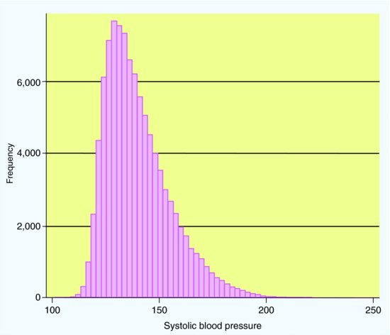
Suppose we have a target population of 100,000 men aged over 65 in one region of the UK. Hypothetically, we could measure the systolic blood pressure of every one of these men. Assume that if we could do this, the true distribution (shown in Figure 4.2) would have a mean of 140 mmHg and a standard deviation of 15 mmHg. Note that the distribution is not Normal – it is skewed to the right, as there are a small number of individuals with very high blood pressures.

Figure 4.2 Histogram of systolic blood pressure in a population of 100,000 men aged > 65 years.

In practice we could not measure the blood pressures for everyone in such a large population. So what happens if we measure the systolic blood pressures in a sample from this population? We randomly selected 100 men from this population, and found that they had a mean blood pressure of 139.3 mmHg, with standard deviation 14.8 mmHg. We carried out this process of sampling 100 men nine more times, obtaining 10 samples in total. The means of these 10 samples were:

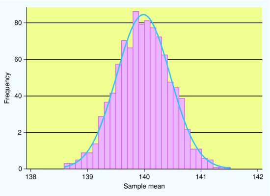
Although none of the sample means is exactly the same as the true population mean (which we know to be 140 mmHg), they are all fairly close to this mean. In order to understand how just one sample can be used to make inferences about the whole population, we need to look at the sampling distribution. This is the distribution the sample means follow if we take lots of samples from the same population. To show this, we repeat this sampling 990 more times (obtaining 1,000 samples in total) and draw a histogram of the sample means (Figure 4.3). Note that the horizontal scale of this histogram is much narrower than that for the histogram of values in the entire population (Figure 4.2). The mean of all the sample means shown in Figure 4.3 is 139.8 mmHg and the standard deviation of all the sample means is 1.49 mmHg.

Figure 4.3 Histogram of sample mean systolic blood pressure from 1,000 samples each of 100 men, from a population of 100,000 men aged > 65 years with a mean systolic blood pressure of 140 mmHg and a standard deviation of 15 mmHg, with a Normal curve superimposed.

This example illustrates three key facts about the sampling distribution of a mean (that is, the distribution of the sample means in a large number of samples from the same population):

So as the sample size gets bigger the standard error of the mean gets smaller – it is a more precise estimate of the population mean. Here the standard deviation of the 1,000 sample means (the standard error) was 1.49 mmHg. This is close to the theoretical value of the standard error for samples of size 100, which (from the above formula) is 15/10 = 1.5 mmHg.

Confidence interval for a population mean

In practice we want to use a mean from a single sample of individuals to make inferences about the value of the true population mean. We know from the example above that the mean of all possible sample means is the true population mean – so we start by using our sample mean as an estimate of the true population mean. We also know from the example above that a single sample mean is unlikely to be exactly the same as the population mean.

Because we know that the distribution of sample means is Normal for large sample sizes, we can say that 95% of the individual sample means are within 1.96 SEs of the mean of this distribution, which is the true population mean (see Chapter 2).

If we transpose this sentence we can say that 95% of the time the true population mean is within 1.96 SEs of the observed sample mean.

In other words the interval from – (1.96×SE ) to + (1.96×SE ) (where is the sample mean) will include the true population mean on 95% of occasions. This interval is known as the 95% confidence interval for the population mean and the values – (1.96×SE ) and + (1.96×SE ) are known as the 95% confidence limits.

The multiplier of 1.96 in the confidence intervals described above was based on the assumption that the sample means follow a Normal distribution. For smaller sample sizes (less than about 50) we have to use a different multiplier, t’, which is derived from the t distribution.

We can calculate a 99% confidence interval, a 90% confidence interval, and so on, in a similar way, by changing the multiplier from 1.96 to 2.58 (99% CI) or 1.64 (90% CI) – these different multipliers are readily available from statistical tables.

Example: Estimating blood pressure (continued)

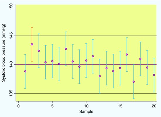
Figure 4.4 shows the point estimates and 95% confidence intervals for 20 different random samples of 100 men, taken from a population with mean blood pressure of 140 mmHg and SD 15 mmHg. Notice that, although the individual 95% confidence intervals vary, 19 out of 20 (i.e. 95%) contain the true population mean of 140. The confidence interval from the second sample (shown with the red bar) does not contain the true value for the population mean.

Figure 4.4 Means (dots) and 95% Confidence intervals (bars) for Systolic Blood Pressure (mmHg) from 20 samples of 100 men each, from a population of 100,000 men aged > 65 with a mean systolic blood pressure of 140 mmHg and a standard deviation of 15 mmHg.

Stay updated, free articles. Join our Telegram channel

Join