where T j denotes the j th time (typically given in months of storage), Y ij denotes the stability limiting response at the j th time for the i th batch, B 0i denotes the intercept for the i th batch, and B 1i denotes the slope for the i th batch. Variation among batches, as exhibited by the variation among batch intercepts and slopes, is accounted for by regarding B 0i and B 1i as random variables. In principle, B 0i and B 1i can have any plausible distribution. Typically, and for the purposes of this discussion, we assume normality. Specifically,
![$$ \left[\begin{array}{c}\hfill {B}_{0i}\hfill \\ {}\hfill {B}_{1i}\hfill \end{array}\right]\sim N\left(\left[\begin{array}{c}\hfill {\beta}_0\hfill \\ {}\hfill {\beta}_1\hfill \end{array}\right],\left[\begin{array}{cc}\hfill {\sigma}_0^2\hfill & \hfill {\sigma}_{01}\hfill \\ {}\hfill {\sigma}_{01}\hfill & \hfill {\sigma}_1^2\hfill \end{array}\right]\right). $$](/wp-content/uploads/2016/07/A330233_1_En_22_Chapter_Equb.gif)
 . Equivalently, we can characterize the process giving rise to the data as
![$$ \left[\begin{array}{c}\hfill {b}_{0i}\hfill \\ {}\hfill {b}_{1i}\hfill \end{array}\right]\sim N\left(\left[\begin{array}{c}\hfill 0\hfill \\ {}\hfill 0\hfill \end{array}\right],\left[\begin{array}{cc}\hfill {\sigma}_0^2\hfill & \hfill {\sigma}_{01}\hfill \\ {}\hfill {\sigma}_{01}\hfill & \hfill {\sigma}_1^2\hfill \end{array}\right]\right) $$](/wp-content/uploads/2016/07/A330233_1_En_22_Chapter_IEq2.gif) . Note that the right-hand side of this description of the process is identical to the linear predictor of a random coefficient linear regression mixed model. Figure 22.1 shows the distribution of expected batch responses under this framework.
. Note that the right-hand side of this description of the process is identical to the linear predictor of a random coefficient linear regression mixed model. Figure 22.1 shows the distribution of expected batch responses under this framework.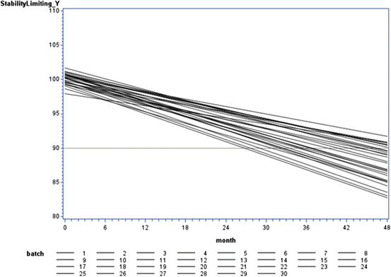
Fig. 22.1
Visualization of variation among batch response over time
To illustrate how this framework extends to more complex models, suppose that the response over time is nonlinear. For example, consider a logistic growth curve
![$$ {Y}_{ij}={B}_{0i}/\left\{1+ \exp \left[-\left({B}_{1i}+{B}_{2i}{T}_j\right)\right]\right\} $$](/wp-content/uploads/2016/07/A330233_1_En_22_Chapter_IEq3.gif) . In this case, B 0i , B 1i and B 2i are batch-specific coefficients. As with the linear case, we account for the inherent variability among batches by regarding B 0i , B 1i and B 2i as random variables. Regardless of the response-over-time model used to describe the process giving rise to the data, the discussion below can be adapted to fit the model’s particulars.
. In this case, B 0i , B 1i and B 2i are batch-specific coefficients. As with the linear case, we account for the inherent variability among batches by regarding B 0i , B 1i and B 2i as random variables. Regardless of the response-over-time model used to describe the process giving rise to the data, the discussion below can be adapted to fit the model’s particulars.Assuming that the regression coefficients are random variables can be controversial, at least in certain cases. The controversy stems, in part, from a misunderstanding of what it means for a process to be in a state of statistical control. The slope of a linear regression illustrates the issue. The process being in a state of statistical control, goes the argument, means that degradation rates do not vary among batches, i.e. no batch-to-batch variability among slopes. However, “in a state of statistical control” does not equate to zero variance. While we hope that the variance is small, strictly speaking it is never zero.
There are, however, situations in which variation among certain batch characteristics is too small to be clinically relevant. Altan et al. (2013) gives examples of products for which variation in the initial response (the intercept) makes sense, but variation in degradation rate (the slope) does not. In such cases, the variance among slopes is indistinguishable from, even if in theory not exactly equal to, zero. Both cases—non-negligible and negligible variance among batch slopes—will be considered as this chapter proceeds.
Continuing with the linear regression, define A as the acceptance criterion. If the stability limiting response increases over time, A will be the value of Y ij above which the product is no longer acceptable; if response decreases over time, A will be the value of Y ij below which the product is no longer acceptable. It follows that the batch-specific shelf life for the i th batch can be determined by solving for the time at which the response,  , i.e. set
  , where T Si denotes the i th batch-specific shelf life. This yields
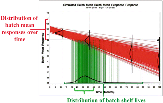
  . Notice that T Si is a random variable whose distribution depends on the distributions of B 0i and B 1i . Figure 22.2 shows the distributions in question: changes in response over time and the resulting shelf life for the batches in the population.
 , i.e. set
  , where T Si denotes the i th batch-specific shelf life. This yields
  . Notice that T Si is a random variable whose distribution depends on the distributions of B 0i and B 1i . Figure 22.2 shows the distributions in question: changes in response over time and the resulting shelf life for the batches in the population.
Fig. 22.2
Visualization of Relationship between Batch Mean and Shelf Life Distributions
Stroup and Quinlan (2010) noted a lack of standardized terminology, stating, “… conversations about shelf life are prone to going astray unless participants take care at the beginning of the discussion to make sure that they agree on a common understanding of all key terminology.” Capen et al. (2012) pursued this point, and provided precise definitions of key shelf life vocabulary. Specifically, with regard to Figs. 22.1 and 22.2, following Capen et al. we use the following terms:
Product distribution: this is the distribution of the observations, Y ij . In the linear regression case, we assume where NI denotes “normally and independently.” Hence, if B 0i and B 1i are uncorrelated,
  . In Figs. 22.1 and 22.2, visualize this as the distribution on the Y-axis.
Shelf life distribution: also called “true shelf life distribution.” This is the distribution of the . Visualize this distribution on the X-axis of Fig. 22.2. Also note that the shelf life distribution is always a consequence of the product distribution
Product shelf life: this is a value on the X-axis that is the target of shelf life estimation. This is the principal controversy of shelf life estimation: what target does one set that addresses the goal stated in the ICH guidance, is realistic, and can be implemented using available statistical methodology? In the next paragraph, we further clarify how statistical science understands and attempts to work with the product shelf life estimation problem.
Figure 22.2 allows us to visualize the goal at the heart of the ICH guidance. Denote T S as the true batch shelf life and  as the estimate of the product shelf life. Strictly speaking, because the distribution of T S is continuous for all
  , setting a shelf life such that all future batches meet the acceptance criterion—i.e. Y ij stays on the correct side of A with probability one for all times
  the stated product shelf life—would require setting
  . This is both impractical and unrealistic. Realistically, a suitable estimate of the product’s shelf life should address two considerations. First, it should provide assurance that most of the distribution of Y ij lies on the acceptance side of A for all times
  , where “most of the distribution” is defined in some agreed upon manner. Second, it would seem reasonable to avoid estimates of shelf life below the effective minimum of the distribution of T S .
 as the estimate of the product shelf life. Strictly speaking, because the distribution of T S is continuous for all
  , setting a shelf life such that all future batches meet the acceptance criterion—i.e. Y ij stays on the correct side of A with probability one for all times
  the stated product shelf life—would require setting
  . This is both impractical and unrealistic. Realistically, a suitable estimate of the product’s shelf life should address two considerations. First, it should provide assurance that most of the distribution of Y ij lies on the acceptance side of A for all times
  , where “most of the distribution” is defined in some agreed upon manner. Second, it would seem reasonable to avoid estimates of shelf life below the effective minimum of the distribution of T S .
Shelf life estimates below the effective minimum of the shelf life distribution risk being undesirable for several possible reasons. For example, if  is below a target—say below 12 months on Fig. 22.2—further development of the product may be discontinued, thus preventing a potentially beneficial product from being made available. Alternatively, an unrealistically short labelled shelf life will cause users to discard and replace the product prematurely. There may be other undesirable contingencies depending on the nature of the product and its intended use.
 is below a target—say below 12 months on Fig. 22.2—further development of the product may be discontinued, thus preventing a potentially beneficial product from being made available. Alternatively, an unrealistically short labelled shelf life will cause users to discard and replace the product prematurely. There may be other undesirable contingencies depending on the nature of the product and its intended use.
Shelf life estimates above an agreed upon target informed by the shelf life distribution also present problems because they would fail to address the primary goal of the ICH guidance, i.e. to provide a time before which the product should be expected to meet acceptance criteria. For example, if the estimated shelf life  exceeds the 5th percentile of the distribution of T S , this in effect means that the probability of a future batch failing to meet the acceptance criterion for the stated life of the product is 5 %. If
  exceeds the 10th percentile of the distribution of T S , the probability of a future batch failing to meet acceptance criteria for the stated life of the product is 10 %. The greater the estimate
  relative to the distribution of T S , the greater the likelihood of a product failing to meet acceptance criteria within its stated shelf life.
 exceeds the 5th percentile of the distribution of T S , this in effect means that the probability of a future batch failing to meet the acceptance criterion for the stated life of the product is 5 %. If
  exceeds the 10th percentile of the distribution of T S , the probability of a future batch failing to meet acceptance criteria for the stated life of the product is 10 %. The greater the estimate
  relative to the distribution of T S , the greater the likelihood of a product failing to meet acceptance criteria within its stated shelf life.
While it is not the purpose of this chapter to prescribe acceptable—or unacceptable—targets for  , the upper and lower thresholds of the distribution of T S described above necessarily play a central role in setting these targets, and, as we shall see below, in evaluating the relative merits and shortcomings of competing methods of obtaining
  .
.
 , the upper and lower thresholds of the distribution of T S described above necessarily play a central role in setting these targets, and, as we shall see below, in evaluating the relative merits and shortcomings of competing methods of obtaining
  .
.This concludes the first aspect of statistical modeling: how did the data arise? In the following sections, we consider the second aspect of modeling—what template do we use to define and estimate relevant parameters and how do we use these estimates to address our objectives?
22.3 Existing Methodology
In this section we describe the methodology Q1E guidelines prescribe for estimating shelf life. Following the ICH Q1E document, we focus on the linear regression case, noting that this approach can be extended to polynomial or nonlinear regression, but the linear regression case is sufficient to illustrate the essential principles involved.
22.3.1 The Q1E Estimation Procedure
As noted in Sect. 22.1, Q1E prescribes linear regression over time based on data from at least three batches. Batches are typically observed at 0, 3, 6, 9 and 12 months initially. Subsequent observations are often taken at 18 and 24 months. Occasionally, there may be additional observations after 24 months, e.g. at 30 or 36 months or even later. Data are then analyzed using the following modeling process:
Analysis begins with an unequal slopes analysis of covariance model:
 where y ijk denotes the k th observation on the i th batch at the j th time, β 0i and β 1i denote the intercept and slope parameters for the i th batch, X j denotes the time (usually in months) when observation at the j th time is taken, and e ijk denotes random variation among observations within a batch, assumed i.i.d. N(0, σ 2). Note that to be technically complete, we should refer to this as an unequal slopes and intercepts model. In the interest of readability, and because this is the only model with unequal slopes allowed under the Q1E guidance, we refer to this model hereafter as the “unequal slopes” analysis of covariance model.

The next step of the Q1E prescribed analysis is the so-called “poolability” step. First, one tests the equal slopes hypothesis,  for all i. That is, are regression slopes equal for all batches? In most cases, the suggested criterion for rejection is
  . The idea here is to use the unequal slopes model unless there is strong evidence for doing otherwise. If we fail to reject the hypothesis of equal slopes, then we test the equal intercept hypothesis, that is,
  for all i.
 for all i. That is, are regression slopes equal for all batches? In most cases, the suggested criterion for rejection is
  . The idea here is to use the unequal slopes model unless there is strong evidence for doing otherwise. If we fail to reject the hypothesis of equal slopes, then we test the equal intercept hypothesis, that is,
  for all i.
Depending on the result of these tests, one of the following three models will be selected:
I.
Unequal Slopes: as given above
II.
Common slope, unequal intercepts: 

III.
Common slope and intercept: 

Subsequent estimation depends on the model selected.
If model I, unequal slopes, is selected, batch-specific 95 % confidence bands are computed for the estimates  . If the response decreases over time, the band whose lower one-sided confidence bound first intersects the acceptance criterion determines the shelf life: the shelf life is the time X at which this intersection occurs.
 . If the response decreases over time, the band whose lower one-sided confidence bound first intersects the acceptance criterion determines the shelf life: the shelf life is the time X at which this intersection occurs.
If model II, common slope, unequal intercepts, is selected, confidence bands for  of the worst batch, that is the batch that intersects the acceptance criterion first, are computed. As before, the shelf life is the time X at which this intersection occurs.
 of the worst batch, that is the batch that intersects the acceptance criterion first, are computed. As before, the shelf life is the time X at which this intersection occurs.
If model III, common slope and intercept, is selected, a confidence band for  is computed. The shelf life is the time X at which the relevant confidence bound intersects the acceptance criterion, A.
 is computed. The shelf life is the time X at which the relevant confidence bound intersects the acceptance criterion, A.
22.3.2 Criticism and Behavior of the Q1E Procedure
We can understand the performance of the Q1E procedure, and why improvements may be needed, by considering two aspects: the procedure’s theoretical shortcomings and its small sample behavior. We examine both in this section.
First, we examine the theoretical. The analysis of covariance model used as the basis of the Q1E procedure is a fixed-batch intercept and slope model. By definition the model does not account for random variation among batch intercepts and slopes. Inference on a fixed-effects model is technically limited to only those levels of the effect actually observed—in this case, inference is technically limited to the three batches in the stability study. It does not apply to other batches in the population—specifically, it does not apply to “all future batches.” Thus, it does not, by definition, address the objectives of shelf life estimation articulated in ICH.
As a practical matter, we know that a mismatch between a model that plausibly describes the process giving rise to the observed data and the model used to analyze the data can lead to inaccurate analysis. In this case, the analysis of covariance model implicitly assumes that all future batches are identical to those observed—that the only source of uncertainty in predicting the behavior of future batches derives from within-batch variability, and no uncertainty whatever comes from between-batch variation. We know that in practice this is an implausible assumption. Variation among batch intercepts and slopes may be small—we assume that it is when the product is in a state of statistical control—but it is never zero.
This raises the second issue: do Q1E’s theoretical limitations translate into problems with its small sample performance that need to be addressed? Quinlan et al. (2013b) and Schwenke (2010) explored the small sample behavior of the Q1E procedure using both simulated data and data provided by industry participants in PQRI’s Stability Shelf Life Working Group. They found that with three batches, the Q1E procedure yielded erratic results, with ample opportunity for both excessively low and excessively high shelf life estimates. Despite the perception that increasing the number of batches increases the likelihood of a lower estimated shelf life, thereby creating a conservative estimate of shelf life, but also a disincentive to collect more data, neither Quinlan nor Schwenke found evidence that this actually happens in practice.
To illustrate their findings, we present below the results from two simulations using parameters that represent a synthesis of intercept and slope characteristics suggested by Altan et al. (2013) and those used by Quinlan et al. and Schwenke in their studies mentioned above. Altan et al. obtained representative intercept and slope characteristics from “33 recent stability trials.” These new simulations not only provide verification of Quinlan et al. and Schwenke’s results, but will allow us to compare the Q1E procedure’s behavior to alternatives proposed in subsequent sections of this chapter.
In the first simulation, one thousand data sets were generated from the process described in Sect. 22.2, with random intercept  , where NI denotes normally and independently distributed, and random slopes
  . These characteristics describe a stability limiting characteristic with an average of 100 at time zero, and a 3 % annual rate of decrease—equivalent to the 0.25 unit decrease per month used as the slope coefficient. Following Quinlan et al. (2013b) and Schwenke (2010) we assume that B 0i and B 1i are uncorrelated. For each simulated data set, observations were generated for each batch at times 0, 3, 6, 9, 12, 18 and 24 months. Thus, each observation was generated as
  , where
  denotes time in months, and
  denotes random variability among observations resulting from analytical variation, measurement error, etc. One set of 1000 simulated experiments was generated with 3 batches per trial, and another set of 1000 was generated with 6 batches per trial. In this simulation, the negative slope indicates that the stability limiting characteristic decreases over time. The acceptance criterion was set at
  , i.e. the product is considered “acceptable” as long as the response is 90 or above.
 , where NI denotes normally and independently distributed, and random slopes
  . These characteristics describe a stability limiting characteristic with an average of 100 at time zero, and a 3 % annual rate of decrease—equivalent to the 0.25 unit decrease per month used as the slope coefficient. Following Quinlan et al. (2013b) and Schwenke (2010) we assume that B 0i and B 1i are uncorrelated. For each simulated data set, observations were generated for each batch at times 0, 3, 6, 9, 12, 18 and 24 months. Thus, each observation was generated as
  , where
  denotes time in months, and
  denotes random variability among observations resulting from analytical variation, measurement error, etc. One set of 1000 simulated experiments was generated with 3 batches per trial, and another set of 1000 was generated with 6 batches per trial. In this simulation, the negative slope indicates that the stability limiting characteristic decreases over time. The acceptance criterion was set at
  , i.e. the product is considered “acceptable” as long as the response is 90 or above.
As mentioned in Sect. 22.2, with some products, while random variation is expected among the B 0i (intercepts), batch-to-batch variation among the B 1i (slopes) may be too small to be clinically relevant, and therefore effectively zero. To assess the behavior of the Q1E procedure and selected alternatives deemed promising in the first simulation, we generated an additional 1000 simulated stability trials with  for all trials (hence no random slope term) and 3 batches per trial.
 for all trials (hence no random slope term) and 3 batches per trial.
Results for the simulated data with non-negligible variance among slopes are discussed from this point through Sect. 22.5. Section 22.6 gives results for the simulated data generated with no random variation among slopes.
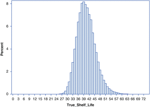
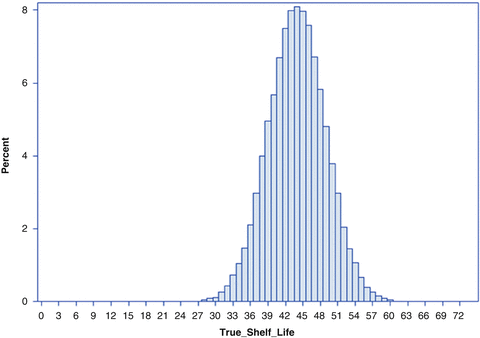
Note that the true shelf life of each simulated batch can be determined as  . Figure 22.3 shows the empirical distribution of true shelf lives for the first simulation, with non-zero variance among slopes. Figure 22.4 shows the empirical distribution for the second scenario, with no random slope effect. Each empirical distribution was created by generating 1,000,000 samples using the parameters given above.
 . Figure 22.3 shows the empirical distribution of true shelf lives for the first simulation, with non-zero variance among slopes. Figure 22.4 shows the empirical distribution for the second scenario, with no random slope effect. Each empirical distribution was created by generating 1,000,000 samples using the parameters given above.
Fig. 22.3
Empirical distribution of true batch shelf with nonzero variation among batch slopes

Fig. 22.4
Empirical distribution of true batch shelf with no variation among batch slopes
Summary statistics important when evaluating the performance of the estimating procedures shown below are as follows. For the first scenario, Fig. 22.3, of the 1,000,000 simulated shelf lives, the lowest was 23.9 months. The 1st percentile of the empirical distribution was 30.3; 5th percentile, 32.9; 10th percentile, 34.3; 25th percentile, 36.9; median, 40.0. The mean of the empirical distribution was 40.4. These percentile values are given in the first column of Table 22.1. Information for the second scenario appears in Table 22.2 and Fig. 22.4. These will be discussed in Sect. 22.6.
Table 22.1
Descriptive statistics for empirical true shelf life distribution and sampling distribution of shelf life estimators
Q1E | Naive_LMM | LCL_RegCoeff | Adj_BLUP | LB_Reg_BLUP | Direct | ||||||||
|---|---|---|---|---|---|---|---|---|---|---|---|---|---|
Quantile | Empirical true shelf life | 3 batches | 6 batches | 3 batches | 6 batches | 3 batches | 6 batches | 3 batches | 6 batches | 3 batches | 6 batches | 3 batches | 6 batches |
Effective Max a | 70 a | 61 | 66 | 44 | 43 | 42.0 | 40.4 | 42.9 | 41.0 | 42.0 | 40.0 | 44 | 41 |
95 % | 49.3 | 42.5 | 44 | 37 | 38 | 35.4 | 36.0 | 36.3 | 36.0 | 35.0 | 34.6 | 38 | 35 |
90 % | 46.9 | 40.5 | 42 | 35 | 37 | 34.1 | 35.1 | 35.2 | 34.7 | 33.8 | 33.8 | 37 | 34 |
75 % Q3 | 43.5 | 38 | 38 | 32 | 35 | 31.9 | 33.5 | 32.9 | 32.8 | 31.6 | 31.4 | 34 | 32 |
50 % Q2 | 40.0 | 35 | 35 | 28 | 34 | 29.3 | 31.6 | 30.4 | 30.0 | 29.0 | 28.8 | 31 | 30 |
25 % Q1 | 36.9 | 32 | 32 | 25 | 32 | 26.8 | 30.1 | 27.7 | 26.6 | 26.4 | 25.4 | 28 | 28 |
10 % | 34.3 | 29 | 30 | 22 | 30 | 24.0 | 28.7 | 24.8 | 24.5 | 23.6 | 23.2 | 25 | 26 |
5 % | 32.9 | 28 | 28 | 20 | 29 | 22.4 | 27.8 | 23.4 | 23.5 | 22.3 | 21.7 | 23 | 25 |
1 % | 30.3 | 25.5 | 25 | 13 | 27 | 18.9 | 26.1 | 20.4 | 21.4 | 18.1 | 15.6 | 21 | 23 |
Effective Min | 24 b | 22 | 23 | 2 | 22 | 11.3 | 25.3 | 16.8 | 19.2 | 6.0 | 6.2 | 17 | 22 |
Mean | 40.4 | 34.9 | 35.6 | 28.4 | 33.7 | 29.2 | 31.8 | 30.2 | 29.7 | 28.8 | 28.4 | 30.7 | 30.1 |
SD | 5.1 | 4.8 | 5.0 | 5.5 | 2.8 | 4.0 | 2.5 | 4.0 | 4.0 < div class='tao-gold-member'>
Only gold members can continue reading. Log In or Register to continue
Stay updated, free articles. Join our Telegram channel
Full access? Get Clinical Tree
 Get Clinical Tree app for offline access

| ||||