Fig. 8.1
Basis for QTiSA-HT cardiac liability assay. The upper panel depicts a ventricular action potential, an electrical response of a ventricular myocyte plotted as the change in transmembrane potential (in millivolts [mV]) across a ventricular membrane in response to an electrical stimulus (at asterisk)). The lower panel depicts the evoked mechanical response of the myocyte, a contraction wave (or twitch), represented as a transient shortening of the myocyte length (measured in micrometers [μm]) that occurs with each action potential). Prolongation of the action potential duration may lead to proarrhythmia, and changes in the extent of myocyte shortening may adversely affect cardiac contractility leading to reducing pump function and hemodynamic effects. QTiSA-HT provides screening information regarding a drugs’ electrophysiologic (proarrhythmic) and contractility liabilities using optical techniques to assess contractions of multiple isolated cardiac myocytes in vitro triggered by electrical stimulation
Using QTiSA-HT, it is possible to characterize concentration-dependent drug effects on ventricular repolarization and contractility based on responses of electrically stimulated myocytes. One challenge of this approach involves applying a so called cumulative dose-response design for data collection. This cumulative design, as compared to individually testing each concentration on a separate set of myocytes, is advantageous for the efficient screening of more compounds in a shorter period of time with fewer myocyte preparations. However due to the nature of this design, observations collected from the same set of the myocytes in a cell chamber are highly correlated because the same myocytes were measured multiple times. This provides a challenge in regards to incorporating within-subject (in this case, the same set of the myocytes in the cell chamber is considered as subject) correlation when analyzing data. Further, since the correlation will be considered in the analysis, it should also be considered when calculating the sample size for experiments. In addition to the within-subject correlation, another challenge involved in the power or sample size evaluation for this experimental design is the day-to-day variability of the assay. Due to differences in myocyte preparations made daily, there is substantial day-to-day variability of measurements even for the control data. The sample size calculation is aiming to detect signal for all future testing compounds which are likely tested in different days. To accommodate this day-to-day variation, a more robust and precise estimation on the assay variance is required for sample size calculations. Finally, to be more effective in guiding the selection of drug candidates early in drug discovery, the biggest challenge for this screening test is that higher throughput experiments, compared to more traditional, manually-based experiments, require automated techniques to provide an early, quick estimate of a safety signal for potential cardiac risk. Statistical approaches to determine the safety signal need to be more robust to control false positive rate in such early stage.
8.3 Cumulative Dose Response Design and Sample Size Calculation
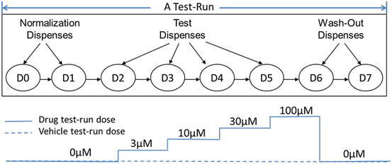
The QTiSA-HT assay follows a cumulative dose-response design (Fig. 8.2) consisting of (a) two recording periods termed dispense 0 [D0] and dispense 1 [D1] which provide baseline parameters, (b) four recording periods (dispenses 2, 3, 4, 5) measuring responses to sequential ascending concentrations of drug (also referred to as time points or dose levels), (c) two recording periods (dispenses 6, 7) assessing drug washout and reversibility of drug effects. The ascending drug concentrations typically used are 3, 10, 30 100 μM concentrations. We call the entire process from dispense 0 to dispense 7 a test-run. Test-runs may be conducted with either drugs or vehicle-control. Each test-run is performed independently in each cell chamber over time. To account for day-to-day variability of the myocyte preparations, the same drug is tested on at least two different days, with a new myocyte preparation made each experimental day.


Fig. 8.2
Cumulative dose response design for QTiSA-HT experiment. A typical “test-run” consisting of two baseline “dispenses” (D0–D1)”, followed by 4 periods of ascending (cumulative) concentrations of test compound (D2–D5) followed by two washout periods (D6–D7). Dispense numbers from D0 to D7 in above diagram represent the time of events during which experimental parameters (representing changes in repolarization or contractility of isolated myocytes) are measured. The total duration of each test-run is 7.5 min, enabling its use in a higher throughput experimental format
For QTiSA-HT experiment, data collected represent repeated measurements at different dispenses (dose levels) from the same experimental preparation (same myocytes cells at the same cell chamber). For example, dispense 2, 3, 4, and 5 is corresponding to dose level 3, 10, 30 and 100 μM, respectively as shown in Fig. 8.2. This cumulative dose-response design saves time (no need to establish baseline values for each concentration tested), saves test compound (using incremental addition to next target concentrations), reduces the number of experimental preparations needed (multiple concentration responses per one preparation), and reduces experimental variability (since same preparation is used to collect the data from all concentrations). Such a design is also useful for biological responses that may not demonstrate stable responses with multiple periods of drug exposures and washout.
On each day, four to eight test-runs recording effects of vehicle-control experiments are performed to supply a concurrent control for all drug test-runs conducted that day. Thus, a typical dataset for screening one drug consists of data collected from 2 days with 6 test-runs per day, involving 2 test-runs for drug and 4 test-runs for vehicle-control. The data collected from vehicle-control are shared amongst all drugs tested that day.
As we discussed in Sect. 8.2, this cumulative design is advantageous for the efficient screening of more compounds in a shorter period of time. However due to the nature of this design, it is quite a challenge when calculating the sample size. The goal of sample size calculation for this particular design is to answer: how many test-runs should be conducted for each drug to have sufficient power to detect a meaningful drug effect? As we discussed above, the current QTiSA platform typically allows at least 4 shared test-runs for control experiments and 2 test-runs for drug per day. Therefore, this sample size calculation is essentially to answer how many days do we need to perform the drug test-runs for screening a same drug? For example, if the answer is 3 days, then in total we will perform 6 test-runs for a screening drug with 2 test-runs performed per day. If a design allows us to conduct 54 runs per day, we can complete the screenings for 25 compounds in 3 days since 50 test-runs for drug can be conducted in each day (the rest 4 test-runs will be reserved for vehicle control). The less the number of days we need, the more compounds we are able to screen and make decision in a fixed time frame.
Statistical test power is the probability of rejecting the null hypothesis when the null hypothesis is false. For example, in our QTiSA experiment, one of the null hypotheses is that there is no concentration-dependent drug effect on cardiac repolarization. Performing power analysis and sample size estimation is an important aspect of any experimental design. Usually, larger sample size provides greater statistical power for a given experimental setting. A good experimental design should provide sufficient power with minimal sample size for the purpose of efficiency. For screening assay, sample size is critical not only to defining statistical power, but also affects assay cost, throughput, and timelines.
There are many ways to calculate the sample size or statistical power for a repeated measurement experimental design. A simple way is to calculate the sample size based on a single time point measurement, usually the most interesting or critical time point. A better approach uses multiple time points after consideration of underlying correlation between time points.
In this screening experiment, the time point or dispense is corresponding to dose concentration level. We are not only interested in testing the drug effect at each dose level, but also interested in testing the dose response trend. Therefore all dose levels are equally important. Sample size calculation based on a single time point, i.e. single dose level, may not provide sufficient power when testing dose response trend. More importantly, because responses to ascending sequential drug concentrations are measured from the same myocytes in this cumulative dose response design, it is obvious that measurements collected from the set of the myocytes at the same cell chamber are correlated over time. From an initial analysis of a large set of control data, the estimated within-subject (here subject is corresponding to the set of the myocytes at the same chamber) correlation is about 0.72 and 0.83 for cardiac repolarization and cardiac contractility respectively. Details about this initial analysis will be discussed later in this section. The high correlations observed from the control data suggest that the within-subject correlation should be considered when calculating the sample sizes as well as analyzing the experimental data. The appropriate statistical method to analyze the experimental data will be discussion in Sect. 8.4.
There are many ways to calculate the sample size when correlation is considered in the setting of repeated measure design. Here we introduce a simple method that can be performed either by theoretic formula or by simulation (Hedeker et al. 1999; Basagana and Spiegelman 2010; Comulada and Weiss 2010). The following four steps describe how to incorporate the correlation when calculating sample size using SAS PROC GLIMMIX procedure (Stroup 2010).
The first step is to estimate the parameters including control means of each variable at each dispense (dispense D2-D5), the overall variance and the correlation coefficient between different dispenses for the same subject, from analyzing the historical control data. This step is a must-done step when performing sample size calculation using any statistical method. A repeated measurement ANOVA model was fitted on a historical control dataset which consists of data collected from a large set of the most recently done control experiments to estimate these parameters. In this model, since the control data includes many days, day is treated as random effect, so the variance component of day can also be estimated from this model. This model is very similar to the one used for testing the drug effect which will be described in Sect. 8.4, but it only applies to the control data and day effect is treated as random.
The second step is to generate “means” data based on the estimated parameters from the first step. According to the experimental design, we typically perform 2 test-runs per day for the same screening compound. Assuming we conduct the experiments for the same compound in m days, then the total number of drug test-runs is 2 m and the total number of the corresponding concurrent control test-runs is 4 m. When using PROC GLIMMIX to do the calculation, the only data we need are the means at each dispense for each group (drug or control) on each day. The overall variance and the correlation coefficient will be provided and held fixed when performing the analysis.
The following example demonstrates how to calculate sample size for testing dose response trend on cardiac repolarization when within-subject correlation is considered. In this example, we assume the day-to-day variation μ day ∼ N (0, 49), and the estimated vehicle-control means at dispenses 2, 3, 4 and 5 is 24, 37, 45 and 50 respectively. These parameter estimations are from step 1. To test dose response trend, we assume the effect size for dispense 5 (high dose) is Δ, the effect size for dispense 2 (low dose) is Δ/4, and the effect sizes for dispense 3 (mid-low dose) and dispense 4 (mid-high dose) are Δ/2. Different dose response relationship can be assumed through different specification on the effect size at each dispense. The SAS code below can generate a series of testing datasets with different Δ range from 0 to 60 ms and different number of days (m = 2, 3 and 4) for the purpose of producing a power curve. A similar procedure can be used to calculate sample size for pair-wise comparison. Notice that the day-to-day variation is also incorporate in the data generation.
The following code only generates one realization of day effect. To account for the randomness of day effect, multiple “means” datasets corresponding to different realizations of day effect should be generated and their resulting sample sizes should be compared. Usually to be more conservative, the largest sample size corresponding to the worst scenario will be used as the final sample size.
data means;
do m=2 to 4 by 1;
do delta=0 to 60 by 1;
do day=1 to m;
dayvar=7*rannor(-1);
do dispense=2 to 5;
z=24*(dispense=2)+37*(dispense=3)+45
*(dispense=4)+50*(dispense=5);
do exp=1 to 6;
id=day*100+exp;
if exp < 5 then trt=0; else trt=1;
y=z+dayvar+delta*(trt=1)*(dispense=2)/4
+delta*(trt=1)*(dispense=3)/2
+delta*(trt=1)*(dispense=4)/2
+delta*(trt=1)*(dispense=5);
output;
end;
end;
end;
end;
end;
drop exp dayvar z;
run;
proc sort; by m delta day id dispense; run;
In step 3, the generated “means” datasets from step 2 are used as the input datasets for the PROC GLIMMIX procedure to output a contrast dataset “contrast” which will be used to calculate power in step 4. The estimated variances and correlation coefficient are specified in the PARMS statement. For both cardiac contractility and repolarization parameters collected from QTiSA-HT assay, we observed that the variances are not homogeneous across dispenses, so we use a first order heterogeneous autoregressive (ARH(1)) covariance structure to analyze the data. This ARH(1) structure will be discussed in Sect. 8.4. For example, the variance at each dispense (dispense 2-5) and the correlation coefficient are held as 89, 315, 232, 239 and 0.72, respectively for testing cardiac repolarization. The PARMS statement with hold option tells the procedure to use the values provided in the statement as the corresponding parameter estimates in the current program. This is why we only need generate “means” data in step 2 and do not need consider the covariance matrix, since it is provided in this PARMS statement. The SAS code for PROC GLIMMIX is provided in the following.
PROC GLIMMIX data=means;
BY m delta;
CLASS day trt dispense id;
MODEL y=day trt dispense trt*day trt*dispense
day*dispense day*dispense*trt;
RANDOM dispense/sub=id type=arh(1) residual;
PARMS 89 315 232 239 0.72 / hold=1,2,3,4,5;
CONTRAST ‘Dose Response’ trt -1 1
trt*dispense -0.1 -0.2 -0.2 -0.5
0.1 0.2 0.2 0.5 ;
ODS OUTPUT contrasts=contrast;run;
Notice that we use the exact same analysis model (Eqs. (8.1)–(8.3) in Sect. 8.4) to output the contract dataset that is subsequently used for power calculation. This is a nice feature of using this procedure to perform power analysis, because the exact same analysis model can be used to perform the power analysis, which is often not feasible using other software. In the CONTRAST statement, we specify the linear coefficients for testing the dose response trend. Different coefficients can be specified through this statement. To keep consistent, the same coefficients should always be used when analyzing the real experimental data.
The last step is to calculate the power based on the “contrast” dataset outputted from step 3. In previous PROC GLIMMIX procedure, a contrast output dataset with number of degree of freedom and F values are generated. This dataset can be used to computer non-centrality parameter, and then we can use probability statements for F-distribution to determine critical value and compute the power. SAS code for the power calculation is provided in the following:
data power;
set contrast;
alpha=0.05;
ncparm=numdf*fvalue;
fcrit=finv(1-alpha,numdf,dendf,0);
power=1-probf(fcrit,numdf,dendf,ncparm);
run;
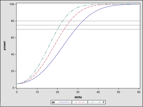
The results based on the above calculation are presented in several power curves (Fig. 8.3). Figure 8.3 shows 3 power curves corresponding to three sample size setting (m = 2, 3 and 4). Figure 8.3 shows that our current 2-day (blue curve with m = 2) experimental design with 2 test-runs of drug experiments and 4 test-runs of control experiments at each day has sufficient power (>=75 %) to detect reasonable dose response trend ( msec at corresponding dose levels) on testing the cardiac repolarization. Similar results on testing cardiac contractility are obtained using the similar procedure. In addition, we also calculated the power for pair-wise comparison at each dose level. The results also support that the two-day design is sufficient. To perform the power analysis for pair-wise comparison at each dose, the similar procedure can be used, except that the contrast statement should be modified to reflect the pair-wise comparison. For example, to test pair-wise comparison between high dose and control, just specify the contrast statement as follows:
 < div class='tao-gold-member'>


 msec at corresponding dose levels) on testing the cardiac repolarization. Similar results on testing cardiac contractility are obtained using the similar procedure. In addition, we also calculated the power for pair-wise comparison at each dose level. The results also support that the two-day design is sufficient. To perform the power analysis for pair-wise comparison at each dose, the similar procedure can be used, except that the contrast statement should be modified to reflect the pair-wise comparison. For example, to test pair-wise comparison between high dose and control, just specify the contrast statement as follows:
Only gold members can continue reading. Log In or Register to continue
Stay updated, free articles. Join our Telegram channel

Full access? Get Clinical Tree


