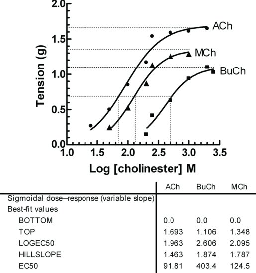
The results in Figure 4.1 can be displayed graphically by plotting the log concentration versus response (Figure 4.2).
Questions
4.2.2 Selective Antagonism
Antagonists that selectively bind to receptor types have been pharmacologically useful in many ways, and have been instrumental in defining types of receptors. As the specificity of antagonists binding to different populations of receptors has been identified, the number of sub-types of receptors has grown. The guinea pig ileum contains both cholinergic receptors (M3) and histamine (H1) on the smooth muscle membrane. Nicotinic receptors are present in the neuronal ganglia. The agonists that selectively bind to the receptors used in this experiment are methacholine, histamine and nicotine. Particular care must be taken in using nicotine, to which tachyphylaxis occurs after repetitive dosing. Tachyphylaxis is a form of short-term desensitization of the nicotinic receptor, and can be thought of as a form of protective response. Tachyphylaxis is common with ion channel receptors, and represents a reversion of the channel to an inactive form after prolonged depolarization, with delayed recovery to the resting state. Rapid repeated stimulation of the receptor results in a decrease in response to the same dose. Responses to stimulation of different receptors can be selectively antagonized by atropine (non-selective muscarinic), diphenhydramine (H1) and hexamethonium (neuronal N).
This experiment is designed to demonstrate the following:
Protocol
Figure 4.3 Typical results obtained for the selective antagonism experiment. (a) Concentration–response curves for methacholine and nicotine. (b) Hexamethonium (10−6 M) inhibited the response to nicotine but did not affect those to methacholine and (c) Atropine (10−6 M) inhibited responses to both methacholine and nicotine.
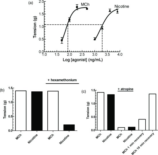
Typical results for this experiment are shown in Figure 4.3.
Questions
4.2.3 Specificity of Blood Cholinesterases
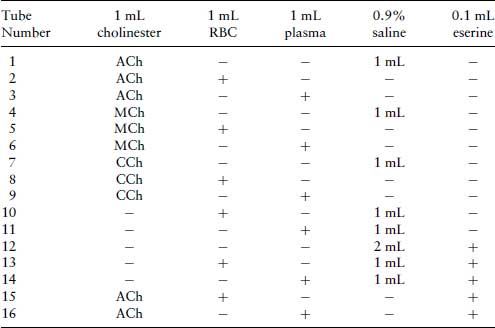
Cholinesterases exist as two isoenzymes: acetylcholine specific cholinesterase (AChE) and the broad specificity butyryl or pseudo-cholinesterase (BuChE or pChE). AChE is bound to the outer post-synaptic membrane and is also found in extraordinarily high concentration within a small portion of the mass of the electroplaques of the organ of the electric eel (Electrophorus electricus). There is also an exceptionally high activity at the neuromuscular junction in the dorsal muscle of the leech (see Section 6.2). pChE has a low specificity and is found in soluble form in blood plasma. It hydrolyses a wide range of cholinesters, and is responsible for the degradation of a number of drugs. An example is the short-term muscle relaxant and depolarizing blocker, succinylcholine, which has a short half-life because it is hydrolysed by pChE. The specificity of these two isoenzymes of cholinesterase can be conveniently demonstrated using blood as a source of both enzymes. AChE is associated with extracellular membrane of red blood cells (RBCs), and, as mentioned, pChE is found in plasma. The specificity of these isoenzymes can be demonstrated by incubating the cholinesters acetylcholine (ACh), methacholine (MCh) and carbachol (CCh) with RBC and plasma and the hydrolysis of the esters monitored by observing the responses of guinea pig isolated ileum. AChE hydrolyses not only ACh, but also pChE. The carbamoyl ester, carbachol, is resistant to hydrolysis by both enzymes.
Protocol
Results
Table 4.1 Preparation of test-tubes for an experiment to demonstrate the specificity of cholinesterases for cholinesters.
Questions
4.2.4 Quantification of the Potency of an Antagonist
This has been introduced in Section 2.1.2. Arunlakshana and Schild (1959) defined a term to describe the potency of an antagonist in terms of the extent to which the antagonist can reduce the potency of an agonist to produce a response. Schild only considered the concentration of the agonist that is required at various antagonist concentrations to produce the same response. He introduced a term pAx, which they defined as the negative log of the concentration of an antagonist that will reduce potency of an antagonist x times. If a tissue is exposed to a competitive antagonist, it will cause a parallel shift of the concentration–response curve to an agonist. The extent to which it shifts the curve is measured by the concentration ratio (CR). This is the concentration of agonist in the presence of antagonist required to produce a fixed response on the linear part of the concentration–response curve divided by the concentration of agonist required to produce the same response in the absence of antagonist. When the antagonist occupies 50% of the receptors, theoretically CR = 2. Schild developed a graphical method to determine a value for −log KB that he termed the pA2 value. The −log value is used to provide a convenient scale for the potency of an antagonist that generally ranges between 5 and 10 (equivalent to concentrations of 10−5–10−10 M). Note that the pA2 value has no units. An experiment is carried out to construct concentration–response curves for an agonist in the absence and presence of at least three concentrations of antagonist. From an equation derived by Gaddum (1937) for the receptor occupancy of an agonist in the presence of a competing, Schild derived an equation relating the CR to KB (the Schild equation):
(4.1) 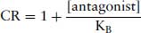
where KB is the equilibrium dissociation constant for the binding of antagonist for the receptor. It is the concentration of antagonist that would occupy 50% of the receptors in the absence of agonist. Theoretically, pKB = pA2
And when expressed as log10,
(4.2) 
so
(4.3) 
(which is in the form of y = mx + c).
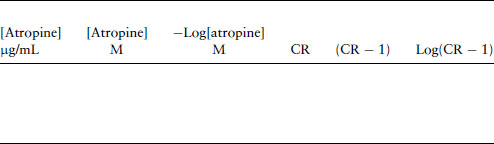
A graph of log[antagonist], (x), against log(CR − 1), (y), should provide a straight line.
For a competitive antagonist, the slope of the line will be 1, and if the negative log[antagonist] is plotted against log(CR − 1) gives a slope of −1. When CR = 2, the antagonist theoretically occupies 50% of the receptor sites, and so log(1) = 0, so the intercept of the line on the x-axis (−log[antagonist]) = pA2. Note that this analysis is only valid when the slope of the Schild plot = −1. The pA2 value describes the potency of an antagonist (the larger the value, the lower the antagonist concentration, and the more potent is the antagonist). This was an early way of defining or classifying receptors. If an antagonist acts on a receptor with the same pA2 value in different tissues, then the receptors in the two sites are defined as being of the same type. For example, atropine would be expected to give the same pA2 value in any location expressing muscarinic receptors, for example, in ileum, heart or trachea. This value is independent of the agonist used as long as it is acting at the same type of receptor as the antagonist.
Protocol
Analysis
Table 4.2 Used to calculate parameters for a Schild plot.
Questions
4.2.5 Bioassays
A bioassay is designed to estimate the concentration or potency of a compound by measuring its biological response (Rang et al., 2012). Bioassays can be used to measure the concentration of a drug, its potency relative to another drug or its binding constant. Whilst many drugs can be measured by analytical chemical techniques, in many cases the exact structure of the drug is not known, or the activity of the drug may not be reflected by analytical chemical techniques (e.g. peptides, isomers, small molecules). Bioassays may be performed in vivo (in living animals) or in vitro. An essential requirement of a bioassay is the availability of a preparation of the test substance of known standard activity. This is not necessarily a pure preparation. In the cases of many biological substances the activity of an unknown can be compared with that of an international standard, and the results expressed as international units (e.g. hormones or other mediators, clotting factors). There are two different types of bioassays – quantal (all-or-none) bioassays and graded bioassays.
Quantal bioassays are where categorical data are obtained and the response is a non-variable end point, such as LD50 or alive or dead. These are best designed and analysed using a contingency table followed by a χ2 test or Fisher’s exact test (see Section 1.6.2).
Graded bioassays. There are three basic designs of graded, quantitative bioassays which can be used to estimate activity with increasing accuracy.
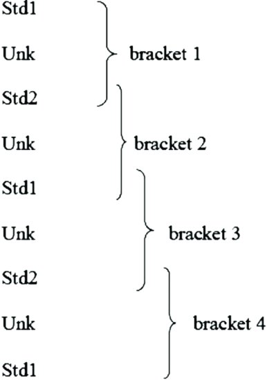
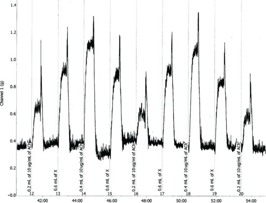
Figure 4.4 A record of responses obtained in a bracketing or three-point assay. The data were recorded using Chart software. (ADInstruments Ltd., U.K.)
Protocol
The guinea pig isolated ileum preparation is set up, as done for the guinea pig isolated ileum preparations described above. Check the maximum response to the standard (add 0.8 mL of 10 μg/mL ACh in the organ bath).
Single-point Assay
So Vunk contains (Cunk × 20) ng of standard (if organ bath volume = 20 mL).
So the concentration of diluted solution of unknown contains: 
(4.4) 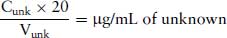
So if the original stock solution of unknown was diluted x times, then the original solution contains (diluted unknown concentration/x) μg/mL.
The design of this assay suffers a great deal of biological variation, and so is inherently inaccurate. This is because the standards and unknown samples were tested over different periods of time. Isolated tissue preparations are notorious for the changes in response over time. The response tends to gradually increase as the tissue recovers from the trauma and changes in temperature occur during the preparation of the tissue. A superior design is the ‘bracketing assay’ as described in the next section.
Bracketing (or three-point) Assay
Select two concentrations of the standard that fall in the linear part of the log concentration–response curve, between 30% and 70% of maximum response to the standard (std1 and std2). Now find a volume of unknown (Vunk) that produces a response approximately midway between these two standard responses (unk). The response to Vunk is bracketed between the responses to std1 and std2. Now repeat these responses in the following order to obtain four overlapping brackets:

A typical record of the results is as shown in Figure 4.4.
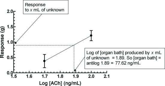
Plot the log concentration against response for each of the brackets, and read off the organ bath concentration obtained when Vunk was added (Figure 4.5).
Figure 4.5 Log concentration against response for std1 and std2. The response for the unknown is read off the abscissa to obtain the log of the bath concentration obtained on addition of Vunk.