The single thresholding depends on the T. This T value determines the intensity range of an object and the intensity range of the image background. For instance, (if the object is brighter than the background) if an pixel intensity value is more than the threshold value, then the pixel will be classified as object; for the pixels which possesses intensity value less than or equal the threshold value, they will be considered as background. This kind of threshold method is considered as ‘threshold above’; another type is ‘threshold inside’ where the object value is in between two threshold values; similarly, another variant is ‘threshold outside’ where the value in between the two threshold values would be classified as background (Shapiro and Stockman 2001).

The efficiency of thresholding technique in segmentation mainly depends on two factors: first factor is the property of the image intensity distribution of both object and background. Thresholding technique performs most efficiently when the intensity of input image has distinct bi-modal distribution without any overlapping range of intensity for object and background (Liyuan et al. 1997). Overlapping range of intensity occurs often due to uneven illumination. Besides, the nature of the object itself can lead to overlapping range in which some regions within the objects in input image has overlapping range of intensity to background. As mentioned in previous chapter, one of the natures of X-ray hand bone radiograph is its uneven illumination throughout the image as well as its overlapping range of intensity distribution among soft tissue region, trabecular bone, and cortical bone due to the nature of hand bone and uneven background illumination as well.

The reasons for the inferior quality of segmented hand bone by thresholding can be summarized as follows:

Another critical problem of single global thresholding is the choice of the threshold value to obtain favorable segmentation result (Baradez et al. 2004). In fact, even the ‘best’ threshold value is selected, the resultant segmented image in the context of hand bone radiograph and in other medical image processing remain inferior. This fact is inevitable due to the nature of global thresholding and the nature of hand bone segmentation: only one threshold. One improvement for this limitation is by adopting multiple global thresholding (Yan et al. 2005). multilevel thresholding classifies the image into multiple classes (>2) (Tsai 1995). The multiple thresholding can represented as follows:
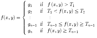
where g _i is group of pixel that represents an object or background. T _i is the threshold values. The f(x, y) is the image pixel intensity in 2D grayscale image in coordination (x, y).

Multiple thresholding might solve the problem arises from the assumption that the input image is of bi-modal type but solve not the problem arises from assumption that the input image is of even illumination. In next subsection, we would review and examine the local/adaptive thresholding that is claimed to be more effective in tackling the problem of uneven illumination.

Adaptive thresholding is segmentation using different thresholds in different sub-images of input image (Zhao et al. 2000). The input image is firstly divided into a number of sub-images; then in each sub-image, suitable threshold is chosen to perform the segmentation, and this process repeats until all sub-images undergo the thresholding segmentation. Adopting different threshold in different region of the input image is proven to be more effective than global thresholding that it is easier to obtain well-separated bi-modal or multiple-modal distributions in the sub-images, and hence, it improves the segmentation result (Shafait et al. 2008). In addition, sub-images are more likely to have uniform illumination implying that as it could resolve the problem that arises from the non-uniform illumination (Huang et al. 2005).

Undoubtedly, it is a fact that adaptive thresholding performs better than global thresholding in tackling the problem of uneven illumination. There are some difficulties in applying the technique effectively in hand bone segmentation due to the problems as follows:

The threshold values are difficult to be set manually as the number of sub-images increases (Buie et al. 2007). In global thresholding as well, the threshold value need to be correctly set in order to optimize the result. We afford to set single global threshold using human inspection. However, when we are dealing with multiple thresholding or adaptive thresholding, automated thresholding is more suitable to decrease repetitive threshold setting by human which is subjective and yet time-consuming. In next subsection, we explore and study about the automated threshold value setting techniques which can be applied in both global thresholding and adaptive thresholding. The implementation of multiple thresholding and adaptive thresholding in hand bone segmentation is illustrated in next subsection using automated threshold values selection to demonstrate that the sole implementation of these technique fail to provide good segmented hand bone.

In global thresholding, each pixel is compared with the global threshold; in local thresholding, each pixel in sub-image is compared with each local threshold which is computed from each sub-image; in dynamic thresholding, each pixel is compared with each dynamic threshold which is computed from sliding a kernel over the input image (Shafait et al. 2008). One of the popular dynamic thresholding methods is Niback method (Niblack 1990).

Generally, dynamic thresholding performs better than global thresholding and local thresholding. However, it has similar drawback as local thresholding that we need to determine the kernel size; the threshold has to be selected manually depending on application. Only suitable selection of kernel size and threshold can produce optimum result of segmentation. In addition, dynamic thresholding consumes much more computational resources relative to local thresholding and global thresholding due to its pixel-wise nature. Besides, in performing the neighborhood operations for dynamic thresholding, the padding problem arises when the kernel approaches the image borders where one or more rows or columns of the kernel are placed out of the input image coordinates.

The main technical issue being frequently discussed is the threshold value selection: the decision to determine the threshold value in which the object and the background could be separated as accurate as possible or the decision to select the threshold value so that the object and the background misclassification rate are lowest. The result of thresholding segmentation process depends heavily on this value. An inaccurate or inappropriate setting of this value will produce disastrous result in thresholding segmentation.

For the choice of threshold value, basically, there are two main methods: the manual threshold selection and the automated threshold selection. Manually determined threshold value heavily relies on human visual system. Threshold value is selected using Visual perception to partition the object from the background; the main drawback of this threshold selection is that it involves human subjective perception toward image quality. Besides, the process itself is extremely time-consuming if the operation involves multiple thresholds. Therefore, it is not practical to determine the threshold value of a large number of images. In short, the manually determined value is not effective.

For automated thresholding method, various methods exist: the simplest method is to utilize the image statistics such as mean, median (second quartile), first quartile, and third quartile, to act as threshold value (De Santis and Sinisgalli 1999): this method performs only relatively well in an image free of noises; the reason is that the noise in the image has influenced the statistic of the image . Typically, if the mean of an image used as threshold value, then it can separate a typical image with object brighter than background into two components; however, while noises exist, the noises have altered the nature that the pixels with intensity more than mean are belonged to the object. Besides, this kind of thresholding method assumes that the object and the background are themselves homogenous. In other words, the object is a group of pixels containing similar pixel intensity; the background is a group of pixels with similar intensity. This assumption has serious limitation especially in medical image segmentation where the target objects like organs or bone are not inherently homogenous. Besides using simple aforementioned statistic in input image, there are other methods to choose the threshold value. In next paragraph, we explore and study different types of automated thresholding techniques that have been developed.

Attributable to the limitations of using simple statistics, various more sophisticated types of thresholding methods based on different techniques in determining the threshold value are proposed: one of the methods is the threshold value selection based on histogram: instead of choosing the mean or median of the image as the threshold value to separate the object and the background, the histogram-based thresholding method determines the threshold value based on the histogram shape assuming that there are distinct range for object and background themselves. The value of a valley point is set as threshold.

In image processing, when the histogram of an image is mentioned, typically we mean a histogram of the values of pixel intensity; the graph of the histogram represents the number of pixels in an image at each intensity value of the pixel in the image. If say in an 8-bit grayscale image, there will be 2⁸ possible values and it means that the histogram shows the occurrence frequency of each intensity in the image. In other words, it is a representation of the image statistics based on the number of the specific intensity’s occurrence.

Histogram analysis is a popular method in automated thresholding (Whatmough 1991). The postulation is that the information obtained from the physical shape of the histogram of the input image signalizes the suitable threshold value in dividing the input image into meaningful regions (Luijendijk 1991). Conventionally, the intensity bin in the valley between peaks is chosen as threshold to reduce the segmentation error rate. Instead of using manual inspections, by only analyzing the shape of the histogram and compute the intensity bin that represents the valley, the relatively good threshold value can be found (Guo and Pandit 1998).

However, the main drawback of this technique is that it depends too heavily on the shape of pixel intensity distribution. Besides, it has no consideration on the pixels location and the pixel surroundings and this leads to the failure in recognizing the semantic of the input image. This method fails when the input image does not have distinctly separated intensity distribution between the foreground and background due to overlapping of intensity as mentioned in last subsection of global thresholding. This category of automatic threshold selection performs thresholding in accordance with the intensity histogram’s shape properties. Utilizing basically the histogram’s convex hull and curvature, the intervening valley and peaks are identified (Whatmough 1991).

This concept is based on the facts that regions with uniform intensity will produce apparent peaks in the histogram. If only the image has distinct peaks on each objects in the images, then multiple thresholding is always applicable via histogram-based thresholding. The favorable shapes of the histogram for the purpose of segmentation are tall, narrow and contain deep valleys. This method is less influenced by the noise, but it has drawbacks like assuming the pixels intensity range of the object and background has a certain degree of distinction. If the image has no distinct valley point in the histogram, this method would fail to separate the object and the background. The main disadvantage of this histogram-based thresholding method is the difficulties they meet when they have to identify the important peaks or valleys in the image used for segmentation and classification. In next paragraph, we would explore another main automated thresholding based on clustering.

The edge-based segmentations discussed in the previous subsection attempt to perform object boundaries extraction in accordance with the identified meaningful edge pixels. Region-based segmentations, on the contrary, seek to segment an image by classifying image into two sets of pixels: interior and exterior, based on the similarity of selected image features. In this subsection, we explore and study several classic methods belong to this category.

The region-based segmentation is based on the concept that the object to be segmented has common image properties and similarities such as homogenous distribution of pixel intensity, texture, and pattern of pixel intensity that is unique enough to distinguish it from other object (Gonzalez and Woods 2007). The ultimate objective is to partition the image into several regions where each region represents a group of pixels belong to a particular object.

Another popular region method is seeded region growing; this method grows from seeds which can be regions or pixels; then, the seeds expand to accept other unallocated pixel as its region member according to some specified membership function (Kang et al. 2012).

In comparison with deformable model-based segmentation, region-based segmentation is considered relatively fast in terms of computational speed and resources. Besides, it is certain that segmentation output is a coherent region with connected edges. Simplicity in terms of concept and procedures is an advantage of region growing for immediate implementation.

Region-based segmentation is insensitive to image semantics; it does not recognize object but only predefined membership function. Besides, the design of the region membership is as difficult as setting a threshold value; region-based segmentation is unable to separate multiple disconnected objects simultaneously. The assumption that the region within a group of object is homogenous has low practical value in hand bone segmentation due to the fact that the bone is formed by cancellous bone and cortical bone that has high variations on texture and intensity range. Besides, in the presence of noise or any unexpected variations, region growing leads to holes or extra-segmented region in the resultant segmented region and thus has low accuracy in certain condition (Mehnert and Jackway 1997). The number and the location of seeds and membership function in seeded region growing, as well as the merging criteria in split–merge region growing, depend on human decisions which are subjective and laborious.

One of the famous region growing methods is the split and merge algorithm; split and merge is an algorithm splitting the image successively until a specified number of regions remain (Tremeau and Borel 1997). To perform the split and merge region growing algorithm, firstly, the entire image is considered within one region. Then, the splitting process begins in the region in accordance with the homogeneity criterion; if the criterion is met, then it splits (Gonzalez and Woods 2007). This splitting process repeats until all regions are homogenous. After the splitting process, the merging process begins. Initially, comparison among neighborhood regions is performed. Then, the region merges to each other according to some criterion such as the pixels’ intensity value where regions that are less than the standard deviation are considered homogenous.

We have reviewed the essential concept of region-based segmentation. The purpose is to identify coherent regions defined by pixel similarities. The main challenge of this type of segmentation is often related to the pixel similarities: what are the features that should be adopted as similarities measurement and how are the thresholds of chosen features should be set in defining the similarity. The selection of features is difficult as they depend on application. For example, if the targeted object is not a connected object, pixel intensity is not suitable as pixel similarities measurement. The setting of threshold is another tricky challenge as it manipulates the trade-offs in terms of flexibility. For example, if the threshold is set too low, the inferior effect of over-segmentation occurs because pixels easily surpass the threshold leading to larger coherent regions than the actual objects; if the threshold is set too high, the otherwise occurs. Region-based segmentation is unable to segment objects of multiple disconnected regions, and therefore, in the context of hand bone segmentation, applying only region-based segmentation is inappropriate as children hand bones for BAA involve different numbers of bones regions at different ages.

Deformable model refers to classes of methods that implement an estimated model of the targeted object using the model constructed by the prior information such as the texture and shape variability of the specific class of object as flexible two-dimensional curves or three-dimensional surfaces. In two-dimensional cases, these curves deform elastically to by satisfying some constraints to match the borders of the targeted object in a given image. The word ‘active’ stems primarily from the nature of the curves in adapting themselves to fit the targeted object. There are three main classes of deformable model: active contour model, active shape model, and AAM.

Deformable models assemble the mathematical knowledge from physics in limiting the shape flexibility over the space, geometry in shape representation, and optimization theory in model-object fitting. These mathematical foundations work together by playing their roles to establish the deformable model. For instance, the geometric representation with certain degree of freedoms is to cover broader shape changes; the principle in physics, in accordance with forces and constraints, controls the changes of shape to permit only meaningful geometric flexibility; optimization theory adjusts the shape to fulfill the objective function constituted by external energy and internal energy; the external energy is associated with the deformation of model to fit the targeted object due to external potential energy, whereas the internal energy constrains the smoothness of the constructed model in terms of internal elasticity forces.

Kass et al. (1988) proposed Active contour model or known as ‘snake’ as a potential solution to segmentation problem (Leymarie 1986). From the perspective of geometry, it is an embedded parametric curve represented as v(s) = (x(s), y(s)) ^T on image plane (x, y) ∊ R ², where x(.) and y(.) denote coordinates functions, and s ∊ [0, 1] denotes the parametric domain. A snake in this context illustrates an elastic contour that fits to some preferred features in image.

To apply active contour model in segmentation, first, establish the initial location of point s in image planes adjacent to targeted object. These points collect ‘evidence’ locally in their territories and feedback to the contour energy. Next, search the update of each point using local information by solving the Euler–Lagrange equation when the contour is in equilibrium according to calculus of variation. Conventionally, numerical algorithm is applied to solve the equation in discrete approximation framework. Lastly, these steps repeat until stopping criteria has been achieved.

Since the active contour model is proposed, a lot of variations have been introduced by scholars. We have summarized some of them which are highly cited as following:

The advantages of active contour compared with previously discussed methods:

Disadvantages of classical active contour model