Chapter 6
Repeated measures data
In this chapter, we consider mixed models approaches to analysing repeated measures data. An introduction to repeated measures data and its analysis is given in Section 6.1. In Section 6.2, covariance pattern models are described, and two worked examples follow in Sections 6.3 and 6.4. Random coefficients models are described in Section 6.5, which is followed by a worked example in Section 6.6. Methods for sample size estimation are introduced in Section 6.7. In this chapter, we will just be considering simple designs where the repeated measures are defined on a single time scale. Occasionally, designs have a more complex pattern of repeated measurements; for example, repeated measurements may be taken within each of several visits. This design will be considered in Section 8.1.
6.1 Introduction
Any dataset in which subjects are measured repeatedly over time can be described as repeated measures data. Repeated measurements can be made either at predetermined intervals (e.g. at fortnightly visits or at specified times following a drug dose) or in an uncontrolled fashion so that there are variable intervals between the repeated measurements. The type of analysis model chosen will depend on whether the intervals are fixed and, if so, whether they are constant.
6.1.1 Reasons for repeated measurements
There are many reasons for collecting repeated measures data. Some examples are as follows:
- To ensure that a treatment is effective over a specified period. Often, this will be done using a carefully planned trial with fixed timings for visits.
- To monitor safety aspects of the treatment over a specified period (repeated efficacy measurements are then incidental).
- To see how long a single dose of a drug takes to become effective by measuring drug concentration or a physiological response at fixed intervals (often over 24 h). In this situation, repeated measurements are taken at a single visit.
- Repeated observations are sometimes inherent in the measurement itself; for example, blood pressure monitors can take measurements as frequently as every 10 s.
- To monitor particular groups of patients over time. Often, these are retrospective studies where repeated measurements have been recorded in an unplanned fashion. For example, repeated observations on patients with a particular disease may be available from a hospital clinic.
- To see how long a single dose of a drug takes to become effective by measuring drug concentration or a physiological response at fixed intervals (often over 24 h). In this situation, repeated measurements are taken at a single visit.
6.1.2 Analysis objectives
The objectives in analysing repeated measures data will differ depending on the purpose of the study. Ideally, they should be clarified at the design stage. Some examples of common objectives are as follows:
- To measure the average treatment effect over time.
- To assess treatment effects at each time point and to test whether treatment interacts with time.
- To assess specific features of the treatment response profile, for example, area under the curve (AUC), maximum or minimum value and time to the maximum value.
- To identify any covariance patterns in the repeated measurements.
- To determine a suitable model to describe the relationship of a measurement with time.
Before considering mixed models, we first review some fixed effects approaches to analysing repeated measures data that are sometimes satisfactory.
6.1.3 Fixed effects approaches
It is important that any analysis of a parallel group study compares treatment effects against a background of between-patient variation. This is because treatment effects are contained within patient effects. Each of these fixed effects approaches has the potential to compare treatments in this way.
Analysis of mean response over time
This method is satisfactory when the overall treatment effect is of interest, the times are fixed and there are no missing data. However, it does not give any information on whether the treatment effect changes over time. When there are missing data, the analysis is only likely to be satisfactory if the response variable does not change with time.
Separate analyses at each time point
Separate analyses are carried out to compare treatments at each time point. Treatment standard errors are then correctly estimated at the between-patient level. One of many drawbacks to this approach is that repeated testing is taking place and therefore a significant treatment effect is more likely to occur at some time point by chance. In addition, the tests will be correlated. There may also be problems of interpretation if a treatment effect is significant at some time points but not at others. Another, admittedly less important, disadvantage is that the treatment standard errors will be less accurate, since they are based only on the observations at one time point, rather than using data from all time points. This analysis strategy is often observed in medical journals, but it is a strategy that should be discouraged.
Analyses of response features
Features summarising each patient’s response profile (e.g. AUC, minimum or maximum value and time to maximum value) can be analysed. This approach is satisfactory if these summary features are of particular interest and if there is not a great deal of missing data. When there are missing data, it may not be possible to obtain a satisfactory estimate of some features (e.g. an AUC estimate would be biased if some of the observations were missing, although it is possible that an approach such as interpolation would help overcome this; the maximum value might be unrepresentative if observations around the true maximum were missing). If summary features are used, then restraint should be exercised in their selection to avoid problems of multiple testing.
Analysis of raw data fitting patient effects as fixed
In this model, patient, treatment, time and treatment·time effects can be fitted as fixed effects. However, treatment standard errors should not be obtained from the residual mean square, since this represents ‘within-patient’ variation. When there are no missing data, standard errors based on between-patient variation can be calculated manually using the patient sum of squares in the ANOVA table (note that many packages such as SAS (PROC GLM) will, by default, calculate treatment standard errors from the residual mean square). When there are no missing data, this model will give identical results to an equivalent random effects model fitting patients as random. It also has the advantage of being able to assess the treatment effects over time. However, it is not appropriate when there are missing data unless special adjustments are made.
6.1.4 Mixed models approaches
Mixed models have the following advantages:
- A single model can be used to estimate overall treatment effects and to estimate treatment effects at each time point. Treatment effects are correctly compared against a background of between-patient variation. There is no need to calculate mean values across all time points (to obtain the overall treatment effects) or to analyse time points separately (to obtain treatment effects at each time point). Standard errors for treatment effects at individual time points are calculated using information from all time points and are therefore more robust than standard errors calculated from separate time points.
- The presence of missing data causes no problems, provided they can be assumed missing at random.
- The covariance pattern of the repeated measurements can be determined and taken account of (e.g. the model can tell us whether the measurements across all time points have a constant correlation or whether the pattern of correlations is more complex and varies with time).
There are several ways a mixed model can be used to analyse repeated measures data. The simplest approach is to use a random effects model with patient effects fitted as random. This will allow for a constant correlation between all observations on the same patient. However, often, the correlation between observations on the same patient is not constant. For example, correlation may decrease as visits become more widely separated in time. A covariance pattern model can be used to allow for this or, alternatively, for a more complex pattern of correlation. These models are considered in Section 6.2. When the relationship of the response variable with time is of interest, a random coefficients model is appropriate. Regression slopes or curves are fitted for each patient, and the regression coefficients are allowed to vary randomly between the patients. These models are considered in Section 6.5.
6.2 Covariance pattern models
The basic structure of covariance pattern models has been described in Section 2.1.5. In this section, we consider their use for analysing repeated measures data in more detail and describe some more complex types of covariance pattern.
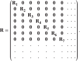
As described in Section 2.1.5, in covariance pattern models, the covariance structure is defined directly by specifying a covariance pattern rather than by using random effects. Observations within each category of a chosen blocking effect (e.g. patients) are assumed to have a specific pattern of covariance, which is defined across a time effect such as period or visit. For example, in a repeated measures trial, a pattern across periods could be specified for covariances between observations occurring on the same patients. The covariance pattern is defined within the residual matrix, R. This matrix is blocked by patients so that only observations on the same patient are correlated. R can be written as

The Ri are submatrices of covariances corresponding to each patient and have dimension equal to the number of observations occurring on each patient. The 0‘s represent matrix blocks of zeros denoting zero correlation between observations on different patients. We will now consider different ways to define covariance patterns in the Ri matrix blocks.
6.2.1 Covariance patterns
A large selection of covariance patterns is available for use in mixed models. Most of the patterns are dependent on measurements being taken at fixed times, and some are also easier to justify when the observations are evenly spaced. There are also patterns where covariances are based on the exact value of time (rather than, say, visit number), and these are most useful in situations where the time intervals are irregular. Some examples of covariance patterns will be given. Still further possible types of covariance patterns can be found in the SAS PROC MIXED documentation.
Simple covariance patterns
Some simple covariance patterns for the Ri matrices for a trial with four time points are shown. In the general pattern (i), sometimes also referred to as ‘unstructured’, the variances of responses,  , differ for each time period i, and the covariances, θjk, differ between each pair of periods j and k. For the first-order autoregressive model (ii), the variances are equal and the covariances decrease exponentially depending on their separation | j − k |, so θjk = ρ|j − k|σ2. This is sometimes an appropriate model when periods are evenly spaced. It can then be seen as a ‘natural’ model from a time series viewpoint. However, it may be justified empirically in circumstances where the observations are not evenly spaced. For example, in monitoring the acute effect of drugs, it is common to take measurements at short intervals soon after drug administration, when the level of observations may be changing rapidly, with increasingly separated intervals later on as observations change more slowly. Under such circumstances, adjoining observations may well show similar covariances, despite unequal periods, with exponentially decreasing covariances for increasingly separated observation numbers.
For the compound symmetry covariance model (iii), all covariances are equal. The Toeplitz model (iv) uses a separate covariance for each level of separation between the time points. This model is also known as the general autoregressive model.
- General

- First-order autoregressive

- Compound symmetry

- Toeplitz

Before software for fitting covariance patterns was readily available, repeated measures analyses were often performed either using a random effects model or by fitting a multivariate normal distribution to the repeated measurements. A random effects model gives identical results to a compound symmetry pattern model (iii) (provided the patient variance component is not negative). Equality of the correlation terms in the compound symmetry structure was often assessed using a test of sphericity (e.g. Greenhouse and Geisser, 1959). However, if a lack of sphericity was found, there were limited alternative analyses available. If the data were complete, then fitting a multivariate normal distribution would give the same results as using a general pattern (i). This model could require a lot of covariance parameters. In addition, if there were missing data, then fitting a multivariate normal distribution would not be satisfactory, as most packages cause all information on patients with incomplete data to be lost. Covariance pattern models overcome these limitations by providing a flexible choice of covariance patterns, which can be fitted to either complete or incomplete data.
Different variances for each time point
Sometimes, variability in a measurement will differ between the time points. This was allowed for in the general covariance pattern (i). Some additional patterns allowing for differing variances are given in the following section. In pattern (v), time points have different variances, but observations on the same patient are uncorrelated. This should only be used if preliminary analyses with more parameterised patterns indicate a lack of correlation between the repeated observations. Patterns (vi)–(viii) have similar forms to the autoregressive, compound symmetry and Toeplitz patterns, except that different variances for each time point are now used.
- Heterogeneous uncorrelated

- Heterogeneous compound symmetry

- Heterogeneous first-order autoregressive

- Heterogeneous Toeplitz

Separate covariance patterns for each treatment group
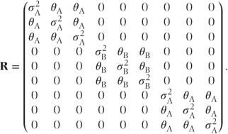
Sometimes, measurements on different treatments will have different variances and covariances. For example, it may be the case that measurements are more variable on an active treatment than on a placebo. This can be allowed for by using separate sets of covariance parameters for each treatment group. For example, if the first three patients in a trial received treatments A, B and A and were each measured at three time points, then the R matrix for these patients with separate compound symmetry structures for each treatment would be

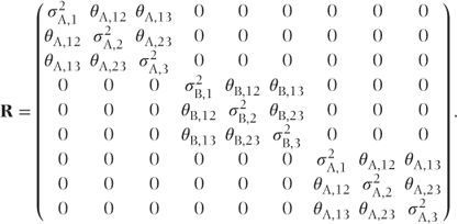
Alternatively, if a general structure was used for each treatment group, then the R matrix would be

Stay updated, free articles. Join our Telegram channel

Full access? Get Clinical Tree


