(1)
Laboratory of General Chemistry and Physical Pharmacy, Ghent University and Centre of Nano- and Biophotonics, Ghent, Belgium
(2)
Laboratory of General Chemistry and Physical Pharmacy, Ghent University, Ghent, Belgium
Abstract
Fluorescence recovery after photobleaching (FRAP) is one of the most useful microscopy techniques for studying the mobility of molecules in terms of a diffusion coefficient. Here, we describe a FRAP method that allows such measurements, relying on the photobleaching of a rectangular region of any size and aspect ratio. We start with a brief overview of the rectangle FRAP theory, and next we provide guidelines for performing FRAP measurements, including a discussion of the experimental setup and the data analysis. Finally, we discuss how to verify correct use of the rectangle FRAP method using test solutions.
Key words
Fluorescence recovery after photobleachingConfocal laser scanning microscopyFluorescence microscopyDiffusion coefficient1 Introduction
Fluorescence recovery after photobleaching (FRAP) has been used extensively to study molecular mobility on a micrometer scale in terms of a diffusion coefficient in a variety of systems like cell membranes [1, 2], polymer gel systems [3–8], and inside living cells [9–12]. FRAP is based on photobleaching of fluorescently labeled molecules, a photochemical process through which fluorescent molecules lose their fluorescence properties after being excited by incoming photons. By illuminating an area in the sample with high-intensity excitation light, the fluorescent molecules within that area are photobleached, leading to a local reduction of fluorescence intensity. A gradual recovery of the fluorescence inside the area occurs due to diffusion of the photobleached molecules outside that area and diffusion of intact fluorescent molecules into that area. The rate of fluorescence recovery is proportional to the rate of diffusion of the fluorescently labeled molecules. Fitting a FRAP model to the observed fluorescence recovery can yield the physical quantities describing the local diffusion in the sample, such as the diffusion coefficient.
By means of a confocal laser scanning microscope (CLSM), it is possible to define a photobleached area of any size and shape and to obtain both spatial and temporal information from the recovery images. However, due to the mathematical complexity, FRAP data analysis remains mostly limited to temporal analysis of the average fluorescence in the photobleached area. In this case, accurate results are only achievable if the initial concentration of bleached molecules after photobleaching is correctly characterized. However, because of nonlinear saturation effects during the highly intense photobleaching, it is very difficult if not impossible to estimate or calibrate the initial bleaching profile exactly [13–16]. One approach to avoid this extra calibration and to increase the accuracy is to take the full spatial and temporal information into account. Recently, we introduced a rectangle FRAP (rFRAP) model that follows this approach [17]. In this model, a rectangular area is assumed instead of the more typical circular region, because this allows to obtain a closed-form expression for the full spatial and temporal recovery process. Moreover, by taking the microscope’s effective photobleaching and imaging resolution into account, the rectangle can have any size and aspect ratio, thus providing for maximum flexibility.
2 Theory
When a rectangle is bleached by a CLSM, it is done sequentially, pixel by pixel and line by line, as is illustrated in Fig. 1.
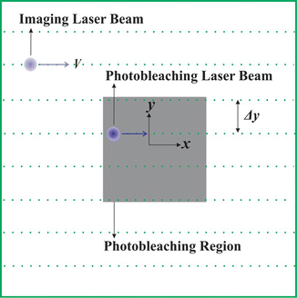
Fig. 1
On a CLSM, it is possible to photobleach a user-defined rectangle with any size and aspect ratio. While scanning in a raster pattern, line by line, the intensity of the laser beam is modulated between a low and high intensity to obtain the user-defined photobleached rectangle
Similar to any analytical FRAP model, in its theoretical derivation, a number of assumptions are made:
1.
3.
For those assumptions, the single-photon 2-D rFRAP model of the fluorescence recovery F(x,y,t) is given by the following formula:
![$$ \begin{array}{lll}\frac{F(x,\ y,t) }{{{F_0}}}=1-\frac{{{K_0}}}{4}\\\qquad\qquad\times\left[ {\mathrm{ erf}\left( {\frac{{x+{l_x}/2}}{{\sqrt{{{r^2}+4{D}t}}}}} \right)-\mathrm{ erf}\left( {\frac{{x-{l_x}/2} }{{\sqrt{{{r^2}+4{D}t}}}}} \right)} \right]\\\qquad\qquad\times \left[ {\mathrm{ erf}\left( {\frac{{y+{l_y}/2 }}{{\sqrt{{{r^2}+4{D}t}}}}} \right)-\mathrm{ erf}\left( {\frac{{y-{l_y}/2}} {{\sqrt{{{r^2} +4{D}t}}}}} \right)} \right] \end{array}$$](/wp-content/uploads/2017/03/A299540_1_En_18_Chapter_Equ00181.gif)
with F 0 being fluorescence before photobleaching, K 0 the amount of photobleaching, l x the length of the bleached rectangle in x-direction, l y the width of the bleached rectangle in y-direction, r 2 the average of the squared lateral imaging and photobleaching resolution, and D the diffusion coefficient. The parameter r takes the finite imaging and effective bleaching resolution into account. Thanks to making use of the full spatial and temporal information in Eq. 2, in practice the parameter r can be determined from the recovery analysis directly without any prior calibration.
(1)
An interesting situation is the combination of a mobile and immobile fraction. Let k be the fraction of mobile molecules, then the fluorescence recovery F k (x,y,t) is given by
![$$ {F_k}(x,y,t)=F(x,y,0)+k\left[ {F(x,y,t)-F(x,y,0)} \right] $$](/wp-content/uploads/2017/03/A299540_1_En_18_Chapter_Equ00182.gif)
where F(x,y,t) is defined by Eq. 1. For more details about the derivation of the general rFRAP expression, we refer to our previous work [17].
(2)
3 Methods
3.1 Experimental Setup and Parameter Settings
1.
A regular (single-photon) CLSM can be used to perform rFRAP experiments. Usually, the intensity of laser scanning is controlled by an AOTF (acousto-optic tunable filter) or a directly modulated laser. The CLSM software typically allows to define a rectangular area in which the intensity of the laser beam is increased to obtain photobleaching. The laser power used for photobleaching also typically is a user-defined setting (see Note 7).
2.
3.
The FRAP sequence should include a number of pre-bleach and post-bleach images (see Note 9). The pre-bleach images will be used to normalize the recovery images in the subsequent data analysis.
A typical sequence of recovery images of a rFRAP measurement is shown in Fig. 2.
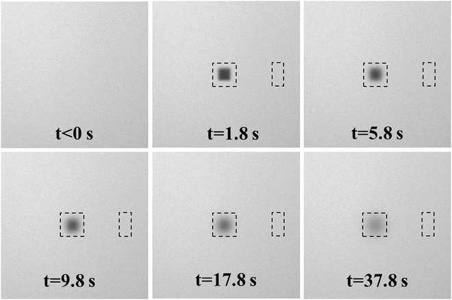
Fig. 2
A typical sequence of recovery images from a rFRAP measurement on a 150 kDa FITC-dextran solution in HEPES buffer at pH = 7.4 with 40 % sucrose. The top left image (t < 0) shows the pre-bleach situation. The next five images show the fluorescence recovery at different times after photobleaching as indicated. The bleach region is 20 μm by 20 μm with the center position at center of the image (256 by 256 pixels). The black dashed square around the bleached region is the region of interest that will be analyzed. The black dashed rectangle to the right of the bleached square shows the region that will be used for background correction (e.g., because of bleaching during imaging or laser fluctuations) in the data analysis
3.2 Data Analysis
The data analysis is done by fitting the rFRAP model (Eqs. 1 and 2) to the pixel values of the recovery images, with the diffusion coefficient (D), the extent of photobleaching (K 0), the fraction of mobile molecules (k), and the average squared resolution (r 2) as free fitting parameters. The fitting procedure can be a simple non-weighted least-squares procedure, or a maximum-likelihood approach for maximum precision [17]. The following steps should be performed:
1.


Before fitting of the data to the rFRAP model, the recovery data should be normalized to the fluorescence before bleaching(see Note 11).
Stay updated, free articles. Join our Telegram channel
Full access? Get Clinical Tree
