is the 100(1-α)th percentile of the F distribution with (2x + 2) and (2n − 2x) degrees of freedom. Then
Table 19.1
Consumer’s and producer’s risk quality points for potential PPQ acceptance sampling plans
Sampling plan Sample size Accept number | Consumer’s risk quality Consumer’s risk = 5 % Quality level corresponding to 5 % probability of acceptance, % defective | Producer’s risk quality Producer’s risk = 5 % Quality level corresponding to 95 % probability of acceptance, % defective |
|---|---|---|
460,0 | 0.649 | 0.011 |
500,0 | 0.597 | 0.010 |
500,1 | 0.945 | 0.071 |
500,2 | 1.25 | 0.163 |
800,0 | 0.374 | 0.006 |
800,1 | 0.591 | 0.044 |
800,2 | 0.785 | 0.102 |
1250,0 | 0.239 | 0.004 |
1250,1 | 0.379 | 0.028 |
1250,2 | 0.503 | 0.065 |
1250,3 | 0.619 | 0.109 |
For other tablet products that are manufactured using a similar process, the estimated defect rate is 0.025 %. The manufacturer will implement for the first time leading indicator (process based) control charts and lagging indicator (product based) control charts to control the components of the process that affects the appearance defect rate.
The tablets were film-coated in a single drum operation; therefore it was deemed appropriate that the samples could be randomly selected at the end of the film coating unit operation. The PPQ acceptance criteria required 3 or less appearance defects in 1250 randomly selected finished product tablets as directed in a plan given in ISO 2859–1:1999 (see Table 19.1). It was determined that four consecutive batches would be used during PPQ. If the process control strategy performs as expected and the defect rate for the process remains at 0.025 %, then there is an approximately 99.96 % probability that any given manufactured batch would meet the (1250, 3) accept criteria. If the process control strategy performed as expected with the leading and lagging indicators associated with the generation of appearance provided significant evidence for process operating in a state of control then there is approximately 99.9 % probability that 4 consecutive batches would pass the (1250, 3) criterion. If the defect rate were still constant but increased to 0.10 % there is a 15 % chance that at least one of the batches would fail during PPQ. Keeping with the same assumptions, there is a 95 % probability that PPQ would fail if the appearance defect rate increased to 0.30 %.
The results of the four batches met the acceptance sampling plan criteria. For Batch 1, Batch 3 and Batch 4 no appearance defects were observed and only one appearance defect was observed in the 1250 inspected for Batch 2. The results from the monitoring of the leading process based indictors (CPPs) and the lagging product based (process output characteristics) demonstrated that the process control strategy performed as expected. Since all relevant data supported that the four batches were manufactured from a consistent and well controlled process, the appearance data was pooled to provide an estimate of the process defect rate and a 95 % one-sided upper confidence bound on the percent non-conforming of the process, 0.02 % and 0.095 %, respectively.
In practice, when multiple characteristics are being assessed from the same sample, for example the 1250 tablets mentioned previously, the acceptance rule would be adjusted to reflect the desired level of quality for each characteristic. For example, Table 19.1 shows 4 different quality levels for a sample size of 1250, and these can be referenced depending on the desired quality level for each characteristic of interest.
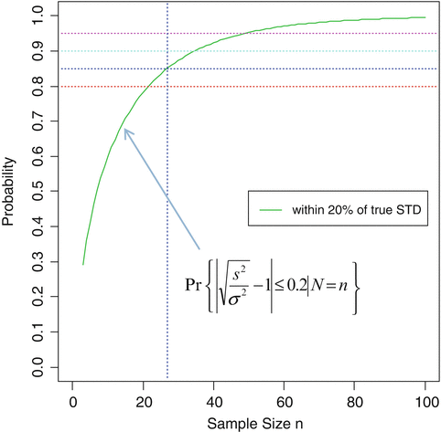
As a result of a successful PPQ, the manufacturer committed to enhanced data collection and evaluation on an additional 25 batches. The number of batches = 25 for enhanced data collection during stage 3A CPV was chosen to provide a high confidence of the batch to batch standard deviation estimate being within a reasonably close interval of the true value. As shown in Fig. 19.1 a sample size of 25 batches provides an (1-α)*100 % = 85 % confidence of yielding an estimate within 20 % of the true value subject to assumptions of normality and independence. Under the normality assumption, the confidence level given by 1-α is calculated by solving for α in the following probability statement for a desired interval of closeness to the true value (defined by r as a proportion of the true value) with degrees of freedom ν (n = number of batches = ν + 1) and s n 2 is an unbiased estimator of σ 2:
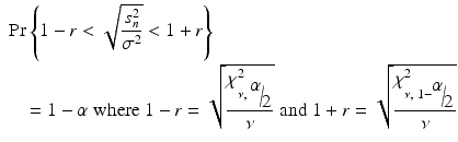 and χ ν,γ 2 is the γth percentile value of the chi-square distribution with ν degrees of freedom.
Fig. 19.1
Probability curve of [0.80 < Ratio of Sample SD to True SD < 1.20] vs sample size under assumption of normality
Similar calculations can be made to reflect levels of risk and closeness to the true value tailored to the product and process as deemed appropriate.
The manufacturer continued enhanced monitoring of the leading and lagging indicators to confirm that the within batch behavior was similar to that observed during PPQ and to better characterize the between batch variation. The conformance to specification plan for the appearance defect, used a single acceptance sampling plan (800, 2) where there was greater than an 85 % probability of failure if the true defect rate exceeded 0.65 % and greater than a 95 % probability of acceptance if the defect rate was less than 0.10 %. If the true appearance defect was appropriately controlled with the leading and lagging indicators at less than 0.025 % then there would be at least a 99 % probability of completing the CPV initial commercial release campaign of 25 batches without a conformance to specification failure.
If success is achieved during the initial CPV stage, the plan for routine commercial release would be to use a double sampling plan. For this double sampling plan, there would be greater than 95 % probability of acceptance for the first tier if the defect rate was less than 0.10 % with a consumer’s risk of less than 10 % if the defect rate was greater than 0.65 %. This coincides with using a sampling plan for a continuing series of lots in the first tier and if failure occurs in the first tier, then switching to an isolated lot test with the consumer’s risk quality of 0.65 % at consumer’s risk of 10 %. An observed failure in the first tier during the CPV routine release stage given a successful initial commercial release CPV would be indicative of a batch defect rate significantly greater than 0.025 %.
The OC Curves for the PPQ, the CPV initial and CPV routine release acceptance sampling plans are provided in Fig. 19.2. After meeting the PPQ acceptance sampling criteria for all four batches, the acceptance sampling plan was changed to inspect 800 units and accept if no more than 2 nonconforming units were observed during the CPV initial commercial release stage. A further reduction in the sample size would be allowed in the routine release stage of CPV, after successfully achieving the requirements for CPV initial commercial release.
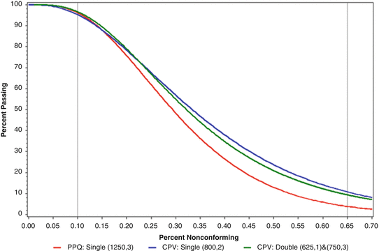
Fig. 19.2
OC curve for comparing PPQ and CPV routine release acceptance sampling plans
19.5.1 Justification for Number of PPQ Batches
The FDA Process Validation guidance section on Stage 2: Process Performance Qualification states “The number of samples should be adequate to provide sufficient statistical confidence of quality both within a batch and between batches. The confidence level selected can be based on risk analysis as it relates to the particular attribute under examination.” This makes explicit the need for a statistical justification of the number of batches chosen for PPQ. It also pertains to how many samples to take to characterize a given batch. These are essentially sample size estimation questions. The usual approach of specifying risks and confidence levels apply but must be refined to address the special circumstances of process validation. We understand risk in this context as the consequence of uncertainties associated with the lack of complete understanding of the product and the process. The remainder of this section will deal with the question of determining and justifying the number of PPQ batches. The question of number of samples to collect for a given batch was discussed in the previous section on acceptance sampling.
The International Society of Pharmaceutical Engineering (ISPE) issued a discussion paper describing three approaches to the question of number of PPQ batches (Bryder et al. 2014). Each approach relates sample size to process and product knowledge and risk levels. These approaches do not represent a consensus position within the industry given how early the industry still is in embracing the principles enunciated in the 2011 guidance. They do form a reasonable starting point for further discussion and evolution. It is also important to emphasize that an assessment of between batch variability is generally not available until Stage 3 of the process validation lifecycle, so the question of number of batches to choose in PPQ is an especially thorny problem.
The ISPE Approach 1 is not based on a statistical argument but rather on judgment regarding the anticipated level of risk of process performance. It allows for 3, 5 or 10 lots corresponding to low, moderate or high levels of risk, respectively.
Approach 2 is based on a target process confidence and capability. It imposes a criterion that observed process capability Cpk ≥ 1. Lewis et al. (2014) showed through simulations that the proposed criterion would be difficult to achieve. For example, if the true Cpk = 1, then there is about a 50 % chance that the observed Cpk will exceed 1, regardless of the number of batches. It was also shown that to achieve an 80 % probability of meeting the criterion with batch sizes of 3,5 and 10, true underlying Cpk’s of about 1.45, 1.35 and 1.25, respectively, would be required. How many pharmaceutical processes can reasonably be anticipated to operate at these levels of capability? Is 80 % adequate for probability of success from a company’s control strategy perspective? If there are multiple CQAs, the proposed criterion is even more difficult to meet.
Approach 3 is based on expected coverage calculated through a property of order statistics. The expected probability that a future observation is between the observed minimum, y(1), and the observed maximum, y(n), is  and n is the total sample size. If there are multiple CQAs, the probability of joint inclusion could be much lower.
and n is the total sample size. If there are multiple CQAs, the probability of joint inclusion could be much lower.None of the ISPE approaches rely on an explicit estimate of batch-to-batch variation or on prior knowledge of process performance expressed through a statistical statement. The latter criticism is particularly important in this context given that the PV guidance 2011 states “The decision to begin commercial distribution should be supported by data from commercial-scale batches. Data from laboratory and pilot studies can provide additional assurance that the commercial manufacturing process performs as expected.” This clearly anticipates a Bayesian approach.
Lewis et al. (2014) proposed a probability of batch success approach to determining and justifying PPQ sample size. The advantages of the method are that it addresses the possibility of multiple CQAs in a natural way and allows a very flexible implementation in both statistical methodology (e.g. frequentist or Bayesian methodology) as well as risk-based approaches. The justification of the PPQ sample size is based on the probability, p, that a batch is within specifications. In this way it imposes no new process performance criteria.
The Bayesian approach with a conjugate prior begins by defining x ∼ Binomial (n, p), where x is the number of batches falling within specification and n is the number of batches manufactured. Let the prior distribution for p be a beta distribution with parameters α and β. In this formulation, α can be thought of as the number of prior successes, β as the number of prior failures, and α + β is the number of prior batches. The non-informative Jeffreys prior uses α = β = ½. The prior mean is α/(α + β). Then it is known that the posterior distribution for p is also a beta distribution, with parameters α′ = α + x and β′ = β + n − x. The posterior predictive distribution is a beta-binomial distribution given by 
where α, β,x and n are as defined previously, and m is the number of PPQ batches to be manufactured. The posterior predictive probability that a single future batch is within specification is (α + x)/(α + β + n).
Given the above Bayesian framework for probability of success of future batches, Fig. 19.3 shows the posterior distributions for 3 successful batches in 3 trials, 5 successful batches in 5 trials, and 10 successful batches in 10 trials.
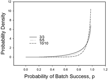
Fig. 19.3
Jeffreys prior and posteriors for 3/3, 5/5 and 10/10 Successes
Let’s consider a hypothetical example. Assume that 10 clinical batches have been successfully manufactured, with no batch failures. Suppose that the goal is to defend the claim of a probability of batch manufacturing success of 0.95 or greater with approximately 80 % confidence. We can use the aforementioned posterior beta distribution to choose increasing values of the parameter n until we achieve the desired confidence level. In this case, 4 additional batches would be necessary with no batch failures, for a total of 14 successful batches in 14 trials. The predictive probability of a future single batch success would be 14.5/15 = 0.967.
Lewis et al. (2014) also provided several “strawman” hypothetical examples of how this approach could be used in practice to justify the number of PPQ batches in relation to risk. These were:
1.
hold lower confidence limit for p constant, vary confidence level with residual risk,
2.
hold confidence level constant, vary lower confidence limit for p with residual risk,
3.
hold parameters of prior distribution constant, vary posterior mean and 0.2 quantile with risk,
4.
hold posterior mean and 0.2 quantile constant, vary prior distribution parameters with risk.
In all the strawman examples, the calculations are with respect to n successful batches of n batches produced. The question of how to assimilate information related to batch failures is an important issue in this context. One should give careful thought to whether the failed batches belong to the population of batches arising from the manufacturing process of interest. If so, some accommodation may be required in the parameters of the prior distribution on p.
An example of strawman model 1 is given in Table 19.2. It gives the number of batches required when holding the lower confidence limit for p approximately constant, and varies the confidence level in relation to risk. The lower confidence limit for p was obtained using the Wilson score procedure.
Table 19.2
Risk level and number of batches in relation to confidence level and lower bound on p when holding the lower confidence limit approximately constant
Risk level | Number batches | Confidence level | pL |
|---|---|---|---|
Minimal | 1 | 0.69 | 0.803 |
Low | 3 | 0.80 | 0.809 |
Moderate | 7 | 0.90 | 0.810 |
High | 11 | 0.95 | 0.803 |
An example of strawman model 2 is given in Table 19.3. It gives the number of batches required when holding the confidence level constant, and varying the lower confidence limit for p in relation to risk. The lower confidence limit for p was obtained using the Wilson score procedure.
Table 19.3
Risk level and number of batches in relation to confidence level and lower bound on p when confidence level is held constant
Risk level | Number batches | Confidence level | pL |
|---|---|---|---|
Minimal | 1 | 0.80 | 0.585 |
Low | 3 | 0.80 | 0.809 < div class='tao-gold-member'>
Only gold members can continue reading. Log In or Register to continue
Stay updated, free articles. Join our Telegram channel
Full access? Get Clinical Tree
 Get Clinical Tree app for offline access

|