CHAPTER 14 Power
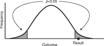
The graphical way to show how we could make an error like this is illustrated in Figure 14-1 by a normally distributed sampling distribution of a sample statistic. If we truly have no treatment effect, then the null hypothesis is true and our test statistic (even though unlikely to occur) did indeed happen. It was our bad luck to get a sample that prompted us to reject the null hypothesis. If this did happen, we would likely be set straight in the future. The results observed in subsequent experiments would not support these original findings, or the results when the treatment is applied in the community would not be as positive.
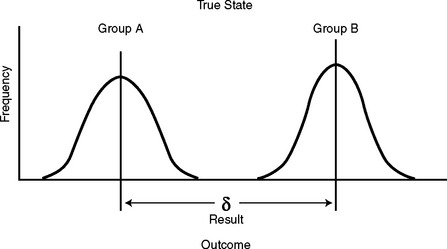
If the treatment really did make a difference, then there are really two different sampling distributions—one for the control group and one for the treatment or alternative group. This is an important concept that explains the essence of statistical tests. The reason we get a difference in results (even accounting for variability among the groups) is that the distributions of the outcome variable are different for each group now that one of them has been changed due to the intervention. This is a complex mathematical way of saying, quite simply, that there is a true difference in outcome due to the intervention.
When we compare two groups that have been exposed to an intervention, we look at the difference in means of the outcome variable of the two groups. This is expressed as δ. The null hypothesis would state the groups are the same, and δ = 0. If the treatment has an effect on the outcome, the means of these groups will be more spread out, as in Figure 14-2. The sample statistic (and resulting test statistic) that we get is not likely to be compatible with the results we would get if the null hypothesis were true.