The administration of drugs by the oral route is noninvasive and very convenient for patients. As a result, it is the most common, and in most situations, the preferred route of drug administration. Several oral dosage forms are available to accommodate the needs of a variety of patients. Solid dosage forms, such as tablets and capsules, are the most common, but liquid dosage forms, including syrups, suspensions, and emulsions, are available to groups of patients, such as children and the elderly, who may have difficulty swallowing solid dosage forms. Despite the popularity of oral dosage forms, they cannot be used in all situations. Some of the major reasons that preclude the oral route include the destruction of a drug by components of the gastrointestinal fluid and/or its inability to pass through the intestinal membrane; extensive presystemic extraction; an immediate drug action is required; the dose must be administered with great accuracy; or the patient is unconscious, uncooperative, or nauseous.

In view of the widespread use of the oral route, it is important to appreciate the unique pharmacokinetic characteristics of oral administration and understand how these may affect drug response. The absorption process brings two additional parameters into the pharmacokinetic model: the bioavailability factor (F) and a parameter for the rate of drug absorption, the first-order absorption rate constant (k_a). Unlike clearance and volume of distribution, these two parameters are properties not only of the drug itself but also of the dosage form, and can vary from one brand of a drug to another.

In this chapter we focus on presenting a pharmacokinetic model for orally administered drugs and discuss how the various model parameters affect the plasma concentration–time profile. The determination of the model parameters and the assessment of bioavailability are addressed. In clinical practice, the absorption parameters (k_a and F) cannot be determined from the limited (1 to 2) samples available from patients. Consequently, the equations for oral administration are not frequently used clinically to individualize doses for patients.

9.2 MODEL FOR FIRST-ORDER ABSORPTION IN A ONE-COMPARTMENT MODEL

9.2.1 Model and Equations

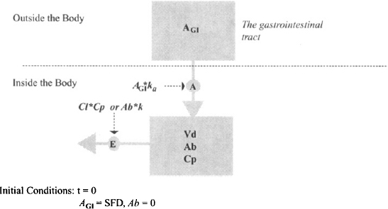
As discussed in Chapter 2, the absorption of drugs from the gastrointestinal tract often follows first-order kinetics. As a result, the pharmacokinetic model can be created simply by adding first-order absorption into the central compartment of the one-compartment model (Figure 9.2). The gastrointestinal tract is represented by a compartment in Figure 9.2. However, since it is outside the body, the body is still modeled as a single compartment. The amount of drug in the gastrointestinal is influenced only by first-order drug absorption:

FIGURE 9.2 Pharmacokinetic model for first-order absorption in a one-compartment model. Ab and A_GI are the amounts of drug in the body and gastrointestinal tract, respectively; k and k_a are the first-order rate constants for elimination (E) and absorption (A), respectively; Cp is the plasma concentration and the concentration of drug in the compartment. The compartment has a volume of Vd, the drug’s volume of distribution; Cl is the clearance; and the effective dose is the product the product of S (salt factor), F (bioavailability factor), and D (the dose administered).

(9.1)

where A_GI is the amount of drug in the gastrointestinal tract and ka is the first-order absorption rate constant. Integrating, we have

(9.2)

where A_GI,0 is the initial amount of drug in the gastrointestinal tract, and is equal to the effective dose (S · F · D):

(9.3)

Equation (9.3) shows that the amount of drug in the gastrointestinal tract starts off at S · F · D and decays to zero by infinity. The speed of the decay is dependent on the first-order rate constant for absorption.

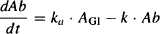
The amount of drug in the body at any time will depend on the relative rates of drug absorption and elimination:

rate of change of the amount of drug in the body = rate of inputs − rate of outputs

(9.4)

Consideration of equation (9.4) provides an explanation for the shape of the plasma concentration–time curve (Figure 9.1). Immediately after drug administration (area A), plasma concentrations increase because the rate of absorption is greater than the rate of elimination. The amount of drug in the gastrointestinal tract is at its maximum, so the rate of absorption is also maximum. In contrast, initially the amount of drug in the body is small, so the rate of elimination is low. As the absorption process continues, drug is depleted from the gastrointestinal tract, so the rate of absorption decreases. At the same time, the amount of drug in the body increases, so the rate of elimination increases. At the peak (B), the rate of absorption is momentarily equal to the rate of elimination. After this time the rate of elimination exceeds the rate of absorption and plasma concentrations fall (area C). Eventually, all the drug is depleted from the intestinal tract and drug absorption stops. At this time (area D) the plasma concentration is influenced only by elimination.

Equation (9.3) can be substituted into equation (9.4), which can then be integrated to yield

(9.5)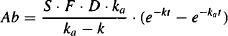

But Cp = Ab/Vd:

(9.6)

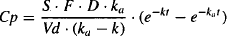
Thus, the plasma concentration at any time after an oral dose is described by a biexponential equation.

9.2.2 Determination of the Model Parameters

The pharmacokinetic model for extravascular administration has four fundamental parameters. Two of the parameters, clearance and volume of distribution, are disposition (elimination and distribution) parameters that are not dependent on the nature of the extravascular dosage form and drug absorption. The other two parameters, the bioavailability factor (F) and the first-order rate constant for absorption (k_a) are functions of both the drug and dosage form. Thus, these parameters can vary from one type and brand of dosage form to another. As always, the one-compartment model has the derived parameter for the rate of elimination (the elimination rate constant and the half-life).

Experimentally the parameters of the model are determined by following a protocol similar to those presented in earlier chapters. Oral doses are administered to a group of individuals, and plasma concentrations are determined at various times after the dose. It is important to obtain several plasma concentration samples around the peak in order to characterize this feature adequately. Data from each person are subject to pharmacokinetic analysis to determine the pharmacokinetic parameters. Each parameter is then averaged across the group to calculate the mean and standard deviation. The basic equation for oral absorption [equation (9.6)] is biexponential and cannot be made linear by transforming the data to the logarithm scale. Generally, pharmacokinetic analysis is conducted using computer software that can perform nonlinear regression analysis to find the model parameters that will most closely match the data observed. However, as was the case with the two-compartment model, the parameters can be obtained by linearizing the data through curve stripping. A discussion of this method helps to demonstrate the importance and influence of each parameter of the model. Additionally, it is a useful procedure to employ if initial estimates of the parameters are needed for computer analysis.

9.2.2.1 First-Order Elimination Rate Constant

At some time after drug administration, the entire dose will have been absorbed and the plasma concentration will decline in a monoexponential manner, due only to first-order drug elimination. Mathematically:

• For extravascular administration, k_a is usually greater than k.
  
• As a result, e^−k_at becomes equal to zero before e^−kt.
  
• When this occurs the equation for the plasma concentration (9.6) reduces to

(9.7)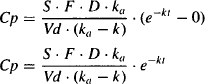

(9.8)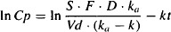

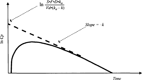
FIGURE 9.3 Plot of logarithm of plasma concentration against time. At later times a linear relationship is observed. The slope of the line is –k and the intercept is ln S · F · D · k_a/[Vd(k_a– k)]

9.2.2.2 Elimination Half-Life

As always, the elimination half-life is calculated from the elimination rate constant:

(9.9)

9.2.2.3 First-Order Absorption Rate Constant

The period before the elimination phase is referred to as the absorption phase. During this period the plasma concentration is under the influence of both absorption and elimination, and the equation is biexponential. Curve stripping is used to separate the two exponential functions during this phase.

To make the equations less cumbersome, let

(9.10)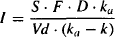

The full expression for Cp [equation (9.6)] is given by

(9.11)

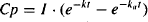
Let the plasma concentration during the elimination phase and its back-extrapolated component be Cp’. Thus,

(9.12)

In the elimination phase, Cp’ = Cp, but in the absorption phase, Cp’ > Cp. Subtracting equation (9.11) from equation (9.12) yields

(9.13)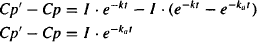

Taking logarithms gives us

(9.14)

This is the equation of a straight line of slope (-k_a) and intercept InI. It is referred to as the feathered line.

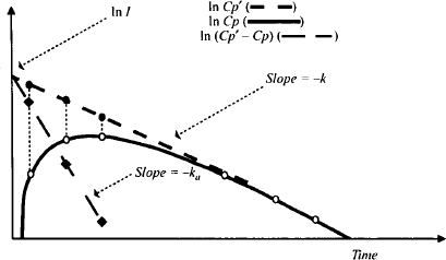
The plot of ln(Cp’ – Cp) is constructed as follows:

FIGURE 9.4 Plot of logarithm of Cp (solid line), Cp’ (upper dashed line), and Cp’ – Cp (broad dashed line) against time. The values of Cp’ (closed circles) that correspond to the time of the given values of Cp (open circles) are noted. ln(Cp’ – Cp) (diamonds) is plotted against time to obtain a straight line of slope –k_a and intercept ln I, where I is S · F · D · k_a/[Vd(k_a – k)].

Stay updated, free articles. Join our Telegram channel

Join