8.2 TISSUE AND COMPARTMENTAL DISTRIBUTION OF A DRUG
8.2.1 Drug Distribution to the Tissues
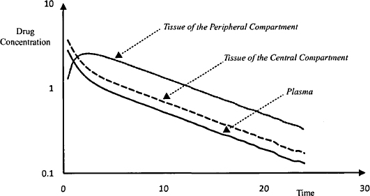
For drugs that display two-compartmental pharmacokinetics, there appear to be two types of tissues with respect to their rate of uptake of drug. One group of tissues, like those of the one-compartment model, take up the drug extremely quickly. The uptake is so rapid that there is no evidence of the distribution based on blood samples taken during the early period after injection. The tissues where this occurs are usually the well-perfused tissues, and the tissue–plasma ratio in these tissues achieves its equilibrium value extremely rapidly and remains constant. Distribution to some other tissues, usually the poorly perfused tissues, occurs more gradually. It is the distribution of the drug to these tissues that is associated with the pronounced initial fall in the plasma concentration. This period is known as the distribution phase (Figure 8.1). Note that drug elimination also occurs during this phase, but it is drug distribution that dominates the fall in the plasma concentration.
In these tissues, where distribution proceeds more slowly, the tissue–plasma concentration ratio increases throughout the distribution phase. Eventually, a type of equilibrium is achieved between the plasma and the poorly perfused tissues. At this time, the distribution phase is complete and the tissue/plasma concentration ratio remains constant. First-order drug elimination then drives the fall in plasma concentration, which as a result falls in a smooth monoexponential manner. This is known as the elimination phase. Figure 8.2 shows how drug concentrations change in hypothetical tissues in both the central and peripheral compartments relative to the plasma concentration. Note that the concentration of drug in both groups of tissues will vary from tissue to tissue. The concentration of drug in a tissue in either compartment could be greater than, less than, or equal to the plasma concentration, depending on factors such as binding and drug transporters.
FIGURE 8.2 Time course of drug concentrations in the plasma and two hypothetical tissues. Note that drug distribution to the tissue of the central compartment (dashed line) appears to be instantaneous and is not visible on the graph. Distribution to the tissue of the peripheral compartment (dotted line) proceeds more slowly and is associated with a sharp fall in concentrations in the plasma (solid line) and tissue of the central compartment.
8.2.2 Compartmental Distribution of a Drug
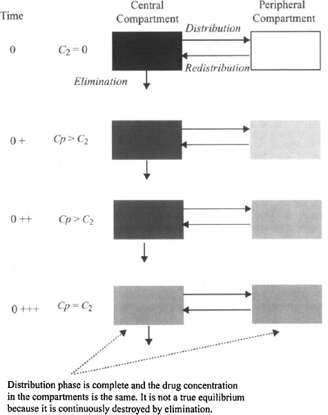
According to the pharmacokinetic model, the body is assumed to consist of two hypothetical compartments (Figure 8.3). The central compartment consists of the plasma and those tissues where drug distribution proceeds very rapidly. By definition the concentration throughout this compartment is equal to the plasma concentration (see Chapter 6). Drug elimination is usually assumed to occur from the central compartment because the organs of elimination are well perfused and are usually part of the central compartment. The second, peripheral compartment consists of those tissues where distribution proceeds more slowly. By definition it is homogeneous and the drug concentration throughout is uniform at all times. Movement between the compartments is assumed to be first-order driven by the amount of drug in a compartment. The movement of drug from the central to the peripheral compartment is referred to as distribution (rate constant k12) and the movement of drug back from the peripheral to the central compartment is referred to as redistribution (rate constant k21). When an intravenous dose is administered, the drug is assumed to undergo instantaneous distribution throughout the central compartment. At this time, the entire dose is present in the central compartment and is distributed throughout the compartment in a completely uniform manner; that is, at any time the drug concentration throughout is the same (Figure 8.4). At time zero, no drug is present in the peripheral compartment. The concentration gradient between compartments then causes a net movement of drug into the peripheral compartment. The concentration in the peripheral compartment increases and the concentration in the central compartment decreases (due to distribution and elimination) (Figure 8.4). Eventually, an equilibrium (pseudo) is achieved, at which time the concentration in the central compartment equals that of the peripheral compartment (Figure 8.4). At this time the concentration in the central compartment decreases due to elimination. As the concentration in the central compartment falls there is a net movement of drug from the peripheral compartment back into the central compartment. The concentration of drug in the peripheral compartment does not correspond to the concentration of drug in any particular tissue that is part of the peripheral compartment. Instead, it represents an averaged concentration of all the tissues that comprise the peripheral compartment. The time course of the distribution process for the two compartments is demonstrated in an interactive video found in the Model, “IV Bolus Injection in a Two-Compartment Model,” at
FIGURE 8.3 Two-compartment model with intravenous bolus injection. Ab, A1, and A2 are the amount of drug in the body, the central compartment, and the peripheral compartment, respectively; Cp is the plasma concentration of the drug and the concentration in the central compartment; C2 is the drug concentrations in the peripheral compartment; V1 and V2 are the respective volumes of the central and peripheral compartments; k10 is the first-order elimination (E) rate constant; k12 and k21 are the rate constants for distribution (D) and redistribution (R), respectively; Cl is clearance; and the effective dose is given by the product of S (salt factor), F (bioavailability factor), and D (the dose administered). Note that for intravenous administration, F = 1.
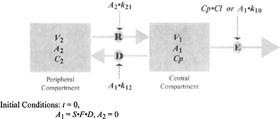
FIGURE 8.4 Relative concentrations of drug in the central (Cp) and peripheral (C2) compartments at different times after intravenous injection in a two-compartment model.
http://www.uri.edu/pharmacy/faculty/rosenbaum/basicmodels.html#chapter8
8.3 BASIC EQUATION
Based on the model shown in Figure 8.3, it is possible to write equations for the rate of change of the amount of drug in the two compartments:
rate of change of the amount of drug in any compartment = rate of inputs − rate of outputs
For the central compartment,
(8.1) 
For the peripheral compartment,
(8.2) 
When these equations are integrated and solved for Cp, the following biexponential solution is obtained:
where α is the hybrid rate constant for distribution, β the hybrid rate constant for elimination, and A and B are the intercepts of the two exponential functions. Thus, according to equation (8.3), the plasma concentration–time profile consists of two exponential terms, A · e−αt and B · e−βt. According to convention, α is always larger than β, and in the vast majority of situations, A · e−αt represents drug distribution and B · e−βt, drug elimination.
8.3.1 Distribution: A, α, and the Distribution t1/2
The function A · e−αt describes the distribution characteristics of a drug during the distribution phase. Note the parameter A, which is an intercept, is dependent on the dose as well as a drug’s pharmacokinetic parameters. The rate constant α is the hybrid rate constant for distribution because although it expresses distribution, it is neither k12 nor k21. It is referred to as a macro rate constant, as it is a complex function of all three of the first-order rate constants (k10, k12, k21) [see equation (8.13)]. The latter first-order rate constants are referred to as the micro rate contants. The half-life determined from a is known as the distribution half-life:
(8.4) 
As distribution is a first-order process, it takes 1 t1/2,α for distribution to go to 50% completion and around 3 to 5 t1/2,α for the distribution phase to go to completion.
8.3.2 Elimination: B, β, and the Beta t1/2
The function B · e−βt describes the characteristics of the plasma concentration–time profile in the elimination phase. The parameter B, like A, is an intercept that is dependent on the dose as well as a drug’s pharmacokinetic parameters. The rate constant β is the hybrid rate constant for elimination and is distinct from the true elimination rate constant k10. It expresses the manner in which the plasma concentration and the amount of drug in the body fall due to drug elimination during the elimination phase. It is also a macro rate constant that is dependent on all three of the micro rate constants (k10, k12, k21) [see equation (8.14)]. The half-life determined from β is referred to as the elimination, biological, or disposition half-life:
(8.5) 
Once the distribution phase is complete, the beta half-life is used to determine how long it will take to eliminate a drug from the body. Since elimination is a first-order process, it will take 1 t1/2,β to eliminate 50% of a dose and around 3 to 5 t1/2,β to eliminate the dose.
Clinically, β or, more specifically, t1/2,β is an important parameter and may be measured in individual patients to optimise therapy. In contrast, α is rarely determined clinically, but it is important to know its approximate value so that the approximate duration of the distribution phase can be determined. This is because when blood samples are collected to determine the t1/2,β, it is important to avoid taking samples in the distribution phase. For example, the elimination half-lives of aminoglycosides such as tobramycin are often measured in patients. These drugs have an t1/2,α of about 5 min. Thus, it is important to wait at least 20 min after an injection before taking blood samples to estimate the t1/2,β. In case of digoxin, which also displays two-compartment pharmacokinetics, the t1/2,α is about 1.5 h. Thus, the distribution phase for digoxin lasts about 6 h.
8.4 RELATIONSHIP BETWEEN MACRO AND MICRO RATE CONSTANTS
The macro rate constants (α and β) and intercepts (A and B) are complex functions of the first-order micro rate constants (k10, k12, k10). The relationship between these parameters is as follows:

(8.7) 
where S is the salt factor and DIV is the value of the intravenous dose. It can be seen in equations (8.8) and (8.9) that A and B are directly proportional to the dose. When the parameters of the two-compartment model are determined experimentally, A, B, α, and β are determined first. These are then used to determine the value of the micro rate constants using the computational formula based on equations (8.6) to (8.9):
(8.11) 

Explicit equations for α and β have also been derived, which allow α and β to be calculated from the micro rate constants:


8.5 PRIMARY PHARMACOKINETIC PARAMETERS
The pharmacokinetic parameters of the model shown in Figure 8.3 consists of first-order rate constants (k10, k12, and k21) and volumes (V1 and V2). As was the case for the one-compartment model, the rate constants are derived, or dependent pharmacokinetic parameters with little direct physiological meaning. The two-compartment model has a total of four primary pharmacokinetic parameters: clearance (Cl), distribution clearance (Cld), volume of the central compartment (V1), and volume of the peripheral compartment (V2). A description of these primary parameters and their relationship to the volume of distribution and the dependent parameters (k10, k12, k21) is presented below.
8.5.1 Clearance
Clearance is consistent with previous definitions: It is a measure of the ability of the organs of elimination to remove drug from the plasma, and it is a constant of proportionality between the rate of elimination at any time and the corresponding plasma concentration. The rate of elimination of a drug can be expressed using either the elimination rate constant (k10) or clearance:
Equating equations (8.15) and (8.16), and given that Cp = A1/V1, the equation can be rearranged to yield
(8.17) 
Clearance can be determined in the usual way from the area under the curve (AUC):
For the two-compartment model the AUC can be calculated:
(8.19) 
8.5.2 Distribution Clearance
The Distribution clearance (Cld) is a measure of the ability of a drug to pass into and out of the tissues of the peripheral compartment. It is determined by the permeability of the drug across the capillary membrane in these tissues as well as the blood flow to the tissues. It can be shown that
where P is the permeability and Qb is the blood flow. It can be seen in equation (8.21) that as the permeability increases, the distribution clearance becomes limited by blood flow. Thus, when a drug is able to diffuse across a membrane with ease, as is the case for most capillary membranes, the distribution clearance will be dependent on the blood flow to a tissue and will be high in those tissues with large blood flows. The distribution clearance is the constant of proportionality between the rate of distribution and the rate of redistribution and the concentration driving the process.
Drug distribution from the central compartment to the peripheral compartment can be expressed using either the first-order rate constant for distribution (k12) or the distribution clearance:
Equating the two expressions in equation (8.22), and substituting for Cp (Cp = A1/V1), it can be written

The rate constant for distribution to the peripheral compartment is derived from the two primary parameters of distribution clearance and the volume of the central compartment.
Drug redistribution from the peripheral compartment back into the central compartment can also be expressed using either distribution clearance or the rate constant for redistribution:
Equating the two expressions in equation (8.24) and substituting for C2 (C2 = A2/V2), it can be shown as

The rate constant for redistribution from the peripheral compartment is derived from the two primary parameters of distribution clearance and the volume of the peripheral compartment. Thus, distribution clearance is a primary pharmacokinetic parameter that determines the values of the rate constants for distribution and redistribution. The rate constants for distribution and redistribution are also determined by V1 and V2, respectively.
When there is equilibrium between the two compartments, the rate of distribution = the rate of redistribution. Thus,
Substituting for k12 and k21 from equations (8.23) and (8.25) yields

Thus, both the ratio k12/k21 [equation (8.26)] and the ratio V2/V1 [equation (8.27)
Stay updated, free articles. Join our Telegram channel

Full access? Get Clinical Tree


