Chapter 8
Other applications of mixed models
In this chapter, the use of mixed models in a variety of situations is considered. In Chapters 5, 6 and 7, we covered three different types of data structure: hierarchical, repeated measures and crossed. Designs with a combination of these features can also arise, and some of these are considered in Sections 8.1–8.4. In Section 8.5, the matched case–control study data are considered, and in Section 8.6, a covariance pattern model is used to allow treatment groups to have different variances in a simple between-patient study. The examples in Sections 8.7–8.14 have arisen from consultancy work and have a variety of structures. In Section 8.15, we look at bioequivalence studies with replicate cross-over designs. The use of mixed models in the analysis of cluster randomized trials is considered in Section 8.16. Section 8.17 looks at the analysis of bilateral data. The chapter finishes in Section 8.18 by looking at the design of incomplete block studies.
8.1 Trials with repeated measurements within visits
Sometimes, repeated measurements occur within visits in cross-over or repeated measures trials. For example, bioequivalence trials often record several blood or urine measurements at each visit within a cross-over design. Studies in cardiology sometimes involve exercise tests where repeated measurements are made throughout the test at each visit. Cross-over trials in asthma may involve a series of lung function measurements made after a ‘challenge’ designed to provoke an asthma attack.
When the data are complete at each visit, a simple approach would be to calculate summary statistics for each visit (e.g. area under the curve, maximum value or time to maximum value) and to analyse these derived variables using methods suggested for ordinary repeated measures or cross-over data (see Chapters 6 and 7). This approach has the advantage of simplicity and gives a straightforward interpretation. It cannot, however, test the treatment·reps interaction (reps are repeated measurements within visits) or always overcome problems caused by missing data.
When there are missing data, the use of summary statistics may not be satisfactory, and a mixed model is often more appropriate. If visits and reps occur at fixed time intervals, a covariance pattern model can be used to structure the covariances by visits and reps. Alternatively, if the visits and/or reps occur at irregular intervals or if it is of interest to model the relationship of the response with time, then a random coefficients model can be used instead.
8.1.1 Covariance pattern models
There are several ways in which the covariance of the data can be modelled when measurements are taken across both visits and reps. In this section, we will present five of the more plausible options. In models for ordinary repeated measures trials (considered in Chapter 6), the overall variance matrix, V, had a block diagonal form, with zero correlations between observations on different patients:
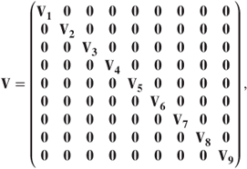
where the Vi are blocks of covariances for observations on the ith patient. We will again use this form for V, but now there are more ways in which the Vi can be structured. We will illustrate a variety of possible structures, assuming a dataset with three visits and three reps per visit (nine observations per patient), which leads to each Vi being a 9 × 9 submatrix.
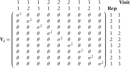
Constant covariances A very simple structure for Vi would assume a constant correlation between all observations on the same patient regardless of the visit or rep number such that
where
- θ = covariance between observations on same patient,
- σ2 = residual variance.
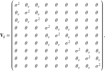
Extra covariance for observations at the same visit The above pattern is perhaps oversimplistic, as it takes no account of the possibility that observations taken at the same visit are more highly correlated than those taken at different visits. A simple way to account for this would be to parameterise Vi with a different covariance for observations on the same visit,
where
- θ = covariance between observations on different visits,
- θv = covariance between observations at the same visit,
- σ2 = residual variance.
A covariance pattern structured by visits Alternatively, it is possible that the correlation between observations is different for each pair of visits leading to
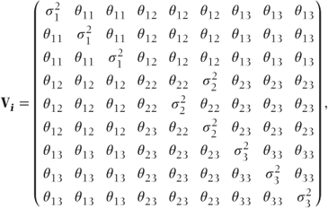
where
- θij = covariance between observations at visits i and j,
 = residual variance at visit i (this may be parameterised as θii + σ2).
This matrix, in fact, has a general covariance pattern structured by visits.
Another alternative would be to use a different covariance pattern for the correlations between visits. For example, by using a Toeplitz pattern, the correlation between observations will depend on the separation of the visits and has the form
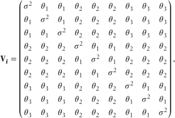
where
- θi = covariance between observations separated by i−1 visits,
- σ2 = residual variance at visit.
A covariance pattern structured by reps It is also possible that correlation between observations at the same visit differs depending on the rep number. A structure assuming constant correlation between observations on different visits (as in (2)) but a different correlation for each pair of reps at the same visit is
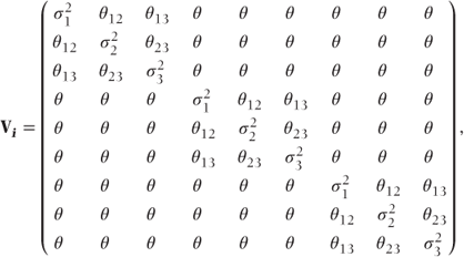
where
- θ = covariance between observations on different visits,
- θij = covariance between observations on reps i and j (at the same visit),
 = residual variance at rep i (this may be parameterised as θii + σ2).
This matrix, in fact, has a general covariance pattern structured by reps (within visits).
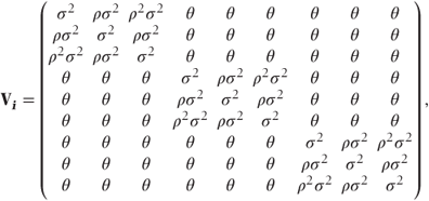
Alternatively, a different pattern from the general pattern could be considered. For example, a first-order autoregressive pattern allowing the correlation between observations to decrease exponentially depending on the separation of the reps would have the form
where
- θ = covariance between observations on different visits,
- ρ|i − j| = correlation between observations on reps i and j,
- σ2 = residual variance.
In both of these models, observations at the same visit could be estimated to be less correlated than those at different visits. This will usually be implausible and can be avoided if we add θ to the covariance of observations at the same visit but with different rep. As we will see in Section 8.1.2, it is this more plausible version of the model that can be implemented in SAS.
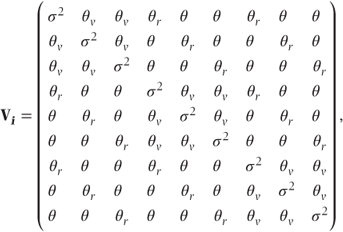
Extra covariance for observations on the same reps It is also possible that there is additional correlation between observations on the same reps. Adding this feature to structure (2) previously shown we obtain the structure
Stay updated, free articles. Join our Telegram channel

Full access? Get Clinical Tree


