of a Modified Moving Least Squares Approximation for Predicting Soft Tissue Deformation Using a Meshless Method

(1)

where m is the number of terms in the basis p(x), and a _i(x) are coefficients that depend on the spatial co-ordinates x. These coefficients are computed by minimizing an error functional defined based on the weighted least squares errors:

$J\left(\mathbf{x}\right)={\displaystyle \sum_{j=1}^n}\left[{\left({u}^h\left({\mathbf{x}}_j\right)-{u}_j\right)}^2w\left(\parallel \mathbf{x}-{\mathbf{x}}_j\parallel \right)\right]$

(2)

where n is the number of nodes in the support domain of x. Rewriting in matrix form yields:

$\mathbf{J}={\left(\mathbf{Pa}-\mathbf{u}\right)}^T\mathbf{W}\left(\mathbf{Pa}-\mathbf{u}\right)$

(3)

Minimization is done by setting the partial derivatives of the error functional J to zero:

$\frac{\partial \mathbf{J}}{\partial \mathbf{a}}={\mathbf{P}}^T\mathbf{W}\mathbf{P}\mathrm{a}\left(\mathrm{x}\right)-{\mathbf{P}}^T\mathbf{W}\mathbf{u}=0$

(4)

Finally, by solving the resulting system of equations, the MLS approximation is obtained as

${u}^h\left(\mathbf{x}\right) = {\displaystyle \sum_{j=1}^n}{\varnothing}_j\left(\mathbf{x}\right){u}_j = {\boldsymbol{\varPhi}}^{\boldsymbol{T}}\left(\mathbf{x}\right)\mathbf{u}$

(5)

where

${\varnothing}_j\left(\mathbf{x}\right)={p}^T\left(\mathbf{x}\right)\left({\boldsymbol{M}}^{\left(-1\right)}\left(\mathbf{x}\right)\boldsymbol{B}\left(\mathbf{x}\right)\right)$

(6)

$\boldsymbol{M}\left(\mathbf{x}\right)={\displaystyle \sum_{j=1}^n}w\left(\mathbf{x}-{\mathbf{x}}_j\right)p\left({\mathbf{x}}_j\right){p}^T\left({\mathbf{x}}_j\right)$

(7)

$\boldsymbol{B}\left(\mathbf{x}\right)=\left[B\left({\mathbf{x}}_1\right)\ B\left({\mathbf{x}}_2\right) \dots B\left({\mathbf{x}}_n\right)\right]$

(8)

$B\left({\mathbf{x}}_1\right)=w\left(\mathbf{x}-{\mathbf{x}}_1\right)p\left({\mathbf{x}}_1\right)$

(9)

Here, u is the nodal vector parameters of all the nodal field variables in the local support domain, Φ(x) is the vector of MLS shape functions and M(x) is known as the moment matrix. Generally, linear or quadratic basis functions and cubic or quartic weight functions are used to create the approximation.

As can be seen from Eq. (6), the shape functions construction depends on the non-singularity of the moment matrix defined by Eq. (7). The necessary conditions for the moment matrix to be non-singular depend on the types of basis functions used. For example, in a two-dimensional case, the moment matrix is non-singular as long as there are at least three non-collinear nodes in the support domain for linear basis functions, whereas for a quadratic basis, at least six nodes are needed in the support domain. The support domain of a point x determines the number of nodes used to compute the approximation value at x. However, some nodal distributions can still lead to singular moment matrices even if enough nodes are included in the support domain. This type of scenario can occur, for example, if the nodes are distributed on two parallel lines in 2D. To overcome this problem, the traditional remedy is to enlarge the support domains in order to include more nodes. This, however, leads to higher approximation error and increased computational cost. Consequently, these limitations prevent the practical use of higher order polynomial basis for randomly distributed nodes despite their potential capability for better approximation of complex deformation fields and better convergence properties.

In this context, Joldes et al. [12] developed a modified MLS with second order polynomial basis. The development of MMLS is based on the observation that a singular moment matrix mainly means that Eq. (4) used to compute the coefficients a(x) has multiple solutions, and therefore the functional (2) does not include sufficient constraints to guarantee a unique solution for the given nodal distribution. Based on this observation, for 2D, additional constraints are included in the functional (2) as

$\overline{J}\left(\mathbf{x}\right)={\displaystyle \sum_{j=1}^n}\left[{\left({u}^h\left({\mathbf{x}}_j\right)-{u}_j\right)}^2\ w\left(\parallel \mathbf{x}-{\mathbf{x}}_j\parallel \right)\right]+{\mu}_{x^2}{a}_{x^2}^2+{\mu}_{xy}{a}_{xy}^2+{\mu}_{y^2}{a}_{y^2}^2$

(10)

where

$\mu =\left[{\mu}_{x^2}\ {\mu}_{xy}\ {\mu}_{y^2}\right]$

(11)

is defined as vector of positive weights for the additional constraints. Using the same minimization procedure, the modified approximant is obtained as:

${\overline{u}}^h\left(\mathbf{x}\right)={\mathbf{P}}^T{\left({\mathbf{P}}^T\mathbf{W}\mathbf{P}+\mathbf{H}\right)}^{-1}{\mathbf{P}}^T\mathbf{W}\mathbf{u}={\displaystyle \sum_{j=1}^n}{\overline{\varnothing}}_j\left(\mathbf{x}\right){u}_j = {\overline{\boldsymbol{\varPhi}}}^{\boldsymbol{T}}\left(\mathbf{x}\right)\mathbf{u}$

(12)

With the new shape function defined as

$\overline{\boldsymbol{\varPhi}}\left(\mathbf{x}\right) = \left[{\overline{\varPhi}}_1\left(\mathbf{x}\right) \dots \kern0.5em {\overline{\varPhi}}_n\left(\mathbf{x}\right)\right] = {\mathbf{P}}^T{\left({\mathbf{P}}^T\mathbf{W}\mathbf{P}+\mathbf{H}\right)}^{-1}{\mathbf{P}}^T\mathbf{W}$

(13)

Here, H is a matrix with all elements zeros except the last three diagonal entries, which are equal to μ

$H=\left[\begin{array}{cc} {\mathbf{O}}_{33} & {\mathbf{O}}_{33} \\ {\mathbf{O}}_{33} & \mathit{diag}\left(\boldsymbol{\upmu} \right) \end{array}\right]$

(14)

and the modified moment matrix is computed as:

$\overline{\mathbf{M}}={\mathbf{P}}^T\mathbf{W}\mathbf{P}+\mathbf{H}=\mathbf{M}+\mathbf{H}$

(15)

The small alteration of the moment matrix presented in the above equation is the only difference between the MMLS and the classic MLS with quadratic basis functions. Nevertheless, it can be shown that the nodal distributions which are admissible for the classical MLS with linear basis functions are also admissible for the presented MMLS [12].

3 Numerical Examples

3.1 Approximation Capability in 2D

To assess the approximations capability of the modified MLS shape functions with quadratic basis, it is compared with classical MLS shape function with linear and quadratic basis. A quartic spline weight function with circular domain was used in the definition of all shape functions:

$$$ w(s)=\left\{\begin{array}{cc} 1-6{s}^2+8{s}^3-3{s}^4, & s\le 1 \\ 0, & s>1 \end{array}\right. $$ ” src=”/wp-content/uploads/2016/10/A321864_1_En_6_Chapter_Equ16.gif”></DIV></DIV><br /> <DIV class=EquationNumber>(16)</DIV></DIV>where <SPAN class=EmphasisTypeItalic>s</SPAN> is the normalized distance<br /> <DIV id=Equ17 class=Equation><br /> <DIV class=EquationContent><br /> <DIV class=MediaObject><IMG alt=$

(17)

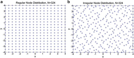
andR _jis the radius of the influence domain of node x _j. In this example, the same weights for all the additional constraints (μ _x² = μ _xy = μ _y² = μ) and a constant radius of influence for all nodes (R _j = R) were used. A 2D rectangular problem domain was defined and the geometry was represented using both regular and irregular node distributions consisting of 324 nodes, as shown in Fig. 1. The irregular nodal distribution consisted of uniformly scattered nodes were obtained by using the Matlab Halton sequence function [13]. The use of this function ensures a uniform nodal density for the problem domain. The following function was used for testing the approximation accuracy in 2D using MLS and the MMLS for different values of μ and R. The function was chosen to present a variety of behaviour in a surface which consists of Gaussian peaks with sharp descent.

$u\left(x,y\right)=x{e}^{-{x}^2-{y}^2}$

(18)

Fig. 1

(a) Regular node distribution, (b) Irregular node distribution

The approximation accuracy was determined using the root mean square error evaluated using a regular distribution of N = 81 × 81 points:

$\mathit{RMSE}=\sqrt{\frac{{\displaystyle {\sum}_{i=1}^N}{\left(u(x)-{u}^h(x)\right)}^2}{N}}$

(19)

The results are shown in Table 1.

Table 1

Root mean square error (RMSE) in approximating $\boldsymbol{u}\left(\boldsymbol{x},\boldsymbol{y}\right)=\boldsymbol{x}{\boldsymbol{e}}^{-{\boldsymbol{x}}^2-{\boldsymbol{y}}^2}$ using 324 nodes with varying radius of nodal influence domain, R