Chapter 2
Normal mixed models
In this chapter, we discuss in more detail the mixed model with normally distributed errors. We will refer to this as the ‘normal mixed model’. Of course, this does not imply that values of the response variables follow normal distributions because they are, in fact, mixtures of effects with different means. In practice, though, if a variable appears to have a normal distribution, the assumption of normal residuals and random effects is often reasonable.
In the examples introduced in Sections 1.1–1.4, we defined several mixed models using a notation chosen to suit each situation. In Section 2.1, we define the mixed model using a general matrix notation, which can be used for all types of mixed model. Matrix notation may at first be unfamiliar to some readers, and it is outwith the scope of this book to teach matrix algebra. A good introductory guide is Matrices for Statistics, Second Edition by Healy (2000). Once grasped, though, matrix notation can make the overall theory underlying mixed models easier to comprehend. Mixed models methods based on classical statistical techniques are described in Section 2.2, and in Section 2.3, the Bayesian approach to fitting mixed models will be introduced. These two sections can be omitted by readers who do not desire a detailed understanding of the more theoretical aspects of mixed models. In Section 2.4, some practical issues related to the use and interpretation of mixed models are considered, and a worked example illustrating several of the points made in Section 2.4 is described in Section 2.5. For those who wish a more in-depth understanding of the theory underlying mixed models, the textbook Mixed Models: Theory and Applications with R, Second Edition by Demidenko (2013) is recommended.
2.1 Model definition
In this section, the mixed model is defined using a general matrix notation that provides a compact means to specify all types of mixed model. We start by defining the fixed effects model, and then extend this notation to encompass the mixed model.
2.1.1 The fixed effects model
All fixed effects models can be specified in the general form

For example, in Section 1.2, Model B was presented as

This model used a subscript i to denote results from the ith patient and a subscript j to denote results on the jth treatment, in the context of a cross-over trial. In the general model notation, however, every observation is denoted separately with a single subscript. Thus, y1 and y2 could represent the observations from patient 1, y3 and y4 the observations from patient 2, and so on. The α terms in the general model will correspond to p1, p2, p3, p4, p5 and p6 and to t1 and t2 and are constants giving the size of the patient and treatment effects. The terms xi1, xi2, …, xi8 are used in this example to indicate the patient and treatment to which the observation yi belongs, and in this case will take the values one or zero. If y1 is the observation from patient 1 who receives treatment 1, x11 then will equal one (corresponding to α1, which represents the first patient effect), x12–x16 will equal zero (as this observation is not from patients 2 to 6), x17 will equal one (corresponding to α7, representing the first treatment effect) and x18 will equal zero. A further example to follow shortly should clarify this notation further.
The above model fits p + 1 fixed effects parameters, α1–αp, and an intercept term, μ. If there are n observations, then these may be written as
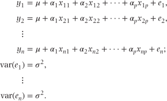
These can be expressed more concisely in matrix notation as

where
- y = (y1, y2, y3, …, yn)′ = observed values,
- α = (μ, α1, α2, …, αp)′ = fixed effects parameters,
- e = (e1, e2, e3, …, en)′ = residuals,
- σ2 = residual variance,
- I = n × n identity matrix.
The parameters in α may encompass several variables. In the above example, they covered patient effects and treatment effects. Both of these are qualitative or categorical variables, and we will refer to such effects as categorical effects. They are also sometimes referred to as factor effects. More generally, categorical effects are those where observations will belong to one of several classes. There may also be several covariate effects (such as age or baseline measurement) contained in α. These relate to variables that are measured on a quantitative scale. Several parameters may be required to model a categorical effect, but just one parameter is needed to model a covariate effect.
X is known as the design matrix and has the dimension n × p (i.e. n rows and p columns). It specifies values of fixed effects corresponding to each parameter for each observation. For categorical effects, the values of zero and one are used to denote the absence and presence of effect categories, and for covariate effects, the variable values themselves are used in X.
We will exemplify the notation with the following data, which are the first nine observations in a multi-centre trial of two treatments to lower blood pressure.
| Centre | Treatment | Pre-treatment systolic BP | Post-treatment systolic BP |
| 1 | A | 178 | 176 |
| 1 | A | 168 | 194 |
| 1 | B | 196 | 156 |
| 1 | B | 170 | 150 |
| 2 | A | 165 | 150 |
| 2 | B | 190 | 160 |
| 3 | A | 175 | 150 |
| 3 | A | 180 | 160 |
| 3 | B | 175 | 160 |
The observation vector y is formed from the values of the post-treatment systolic blood pressure:

If pre-treatment blood pressure and treatment were fitted in the analysis model as fixed effects (ignoring centres for the moment), then the design matrix would be
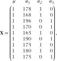
where the columns of the design matrix correspond to the parameters

We note in this case that the design matrix, X, is overparameterised. This means that there are linear dependencies between the columns, for example, we know that α3 will be zero if α2 = 1 and one if α2 = 0. X could alternatively be specified omitting the α3 column to correspond with the number of parameters actually modelled. However, the overparameterised form is used here since it is used for specifying contrasts by SAS procedures such as PROC MIXED (this procedure will be used to analyse most of the examples in this book).
V is a matrix containing the variances and covariances of the observations. In the usual fixed effects model, variances for all observations are equal, and no observations are correlated. Thus, V is simply σ2I.
2.1.2 The mixed model
The mixed model extends the fixed effects model by including random effects, random coefficients and/or covariance terms in the residual variance matrix. In this section, the general notation will be given, and in the following three sections, the specific forms of the covariance matrices for each type of mixed model will be specified.
Extending our fixed effects model to incorporate random effects (or coefficients), the mixed model may be specified as

for a model fitting p fixed effects parameters and q random effects (or coefficients) parameters. It will be recalled from Chapter 1 that random effects are assumed to follow a distribution, whereas fixed effects are regarded as fixed constants. The model can be expressed in matrix notation as

where y, X, α and e are as defined in the fixed effects model, and

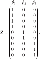
Z is a second design matrix with dimension n × q giving the values of random effects corresponding to each observation. It is specified in exactly the same way as X was for the fixed effects, except that an intercept term is not included. If centres were fitted as random in the multi-centre example given previously, the β vector would then consist of three parameters, β1, β2 and β3, corresponding to the three centres, and the Z matrix would be
Alternatively, if both the centre and the centre·treatment effects were fitted as random, then the vector of random effects parameters, β, would consist of the three centre parameters, plus six centre·treatment interaction parameters β4, β5, β6, β7, β8 and β9. The Z matrix would then be
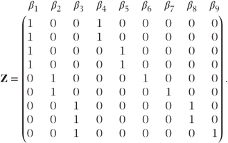
Again, note that this matrix is overparameterised due to linear dependencies between the columns. It could alternatively have been written using four columns: 3 − 1 = 2 for the centre effects and (3 − 1) × (2 − 1) = 2 for the centre·treatment effects.
Covariance matrix, V
We saw in the fixed effects model that all observations have equal variances, and the observations are uncorrelated. This leads to the V matrix being diagonal. When random effects are fitted, we saw in Section 1.2 that this results in correlated observations. In the context of the cross-over trial, we saw that observations on the same patient were correlated (with covariance equal to the patient variance component), while those on different patients were uncorrelated. We now generalise this result, using the matrix notation.
The covariance of y, var(y) = V, can be written as

Since we assume that the random effects and the residuals are uncorrelated,

Since α describes the fixed effects parameters, var(Xα) = 0. Also, Z is a matrix of constants. Therefore,

We will let G denote var(β), and since the random effects are assumed to follow normal distributions, we may write β ∼ N(0, G). Similarly, we write var(e) = R, the residual covariance matrix, and e ∼ N(0, R). Hence,

In the following three sections, we will define the structure of the G and R matrices in random effects models, random coefficients models and covariance pattern models.
2.1.3 The random effects model covariance structure
The G matrix
The dimension of G is q × q, where q is equal to the total number of random effects parameters.
In random effects models, G is always diagonal (i.e. random effects are assumed uncorrelated). If just centre effects were fitted as random in the simple multi-centre example with three centres, then G would have the form

where  is the centre variance component. If both centre and centre·treatment effects were fitted as random, then G would have the form
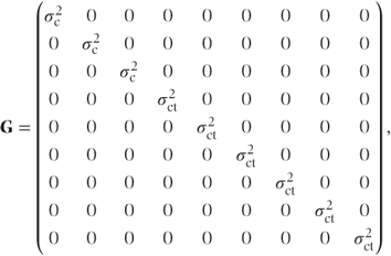
where  is the centre·treatment variance component.
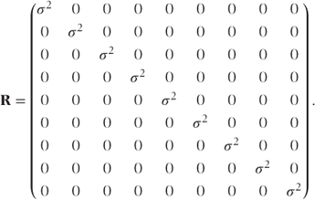
The R matrix
The residuals are uncorrelated in random effects models and R = σ2I:
The V matrix
We showed earlier that the variance matrix, V, has the form V = ZGZ′ + R.
ZGZ′ specifies the covariance due to the random effects. If just centre effects are fitted as random, then we obtain
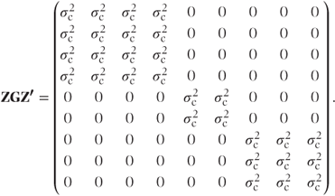
This matrix could be obtained by the laborious process of matrix multiplication but it always has the same form. It has a block diagonal form with the size of blocks corresponding to the number of observations at each random effects category. The total variance matrix, V = ZGZ′ + R, is then

This also has a block diagonal form with the covariances for observations at the same centre equal to the random effects variance component,  , and variance terms on the diagonal equal to the sum of the centre and residual variance components,
  . (We note that this corresponds to the results from the cross-over trial example introduced in Section 1.2, where the random effect was patient rather than centre.) If both centre and centre·treatment effects had been fitted as random, then
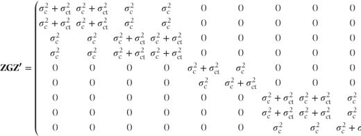
and
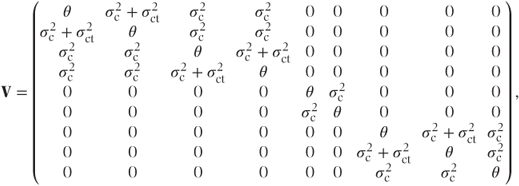
where  . Thus, V again has a block diagonal form with a slightly more complicated structure. The centre·treatment variance component is added to the covariance terms for observations at the same centre and with the same treatment.
2.1.4 The random coefficients model covariance structure
The statistical properties of random coefficients models were described in the repeated measures example introduced in Section 1.4. We will define their covariance structure in terms of the general matrix notation we have just introduced for mixed models. Random coefficients models will be discussed in more detail in Section 6.5.
The following data will be used to illustrate the covariance structure. They represent measurement times for the first three patients in a repeated measures trial of two treatments.
| Patient | Treatment | Time (days) |
| 1 | A | t11 |
| 1 | A | t12 |
| 1 | A | t13 |
| 1 | A | t14 |
| 2 | B | t21 |
| 2 | B | t22 |
| 3 | A | t31 |
| 3 | A | t32 |
| 3 | A | t33 |
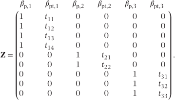
If patient and patient·time effects were fitted as random coefficients, then there would be six random coefficients. We will change notation from Chapter 1 for ease of reading to define these as βp, 1, βpt, 1, βp, 2, βpt, 2, βp, 3 and βpt, 3, allowing an intercept (patient) and slope (patient·time) to be calculated for each of the three patients. The Z matrix would then be
Stay updated, free articles. Join our Telegram channel

Full access? Get Clinical Tree


