Chapter 3
New Product Forecasting
If a man gives no thought about what is distant he will find sorrow near at hand.
Confucius
A fact poorly observed is more treacherous than faulty reasoning.
Paul Valery
Chapter 2 discussed the alignment of forecasting methodologies with a product’s position in its lifecycle. New product forecasting covers the evaluation of a product that still is in development (that is, prior to the product’s launch in the marketplace). This chapter presents the process, tools, methods, and algorithms used in new product forecasting.
Tools and Methods
In Chapter 2 we discussed the tools and methods applicable for product forecasting, and identified the ‘judgment rich’ methods as those most applicable to new product forecasting. These tools are represented by the ‘Judgment’ and ‘Counting’ columns in Figure 2.7.
New Product Forecast Algorithm
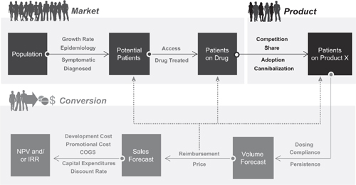
The general forecast algorithm used in new product forecasting is presented in Figure 3.1. This algorithm, or simple variations thereof, can be generalized to almost all new product forecasting exercises. The level of detail varies as the forecast needs become more complex, but the same logic flow applies at all points in a product’s life cycle. The algorithm can be divided into three components, representing the elements required to model the market, to forecast the product, and to convert patients on product into revenue. These structural divisions – market, product, and conversion – form the logical division of market dynamics in new product forecasting.
Figure 3.1 Generalized new product forecast algorithm
Modeling the Market
Modeling the market determines the potential market size for new products. It is a measure of potential and represents the theoretical maximum use for a product. Each market is defined by the user depending upon the dynamics to be forecast in the market. In the simplest example, the forecaster defines the market as those products that compete against each other in the prescription drug market for a specific disease state. Alternatively, this definition can be expanded to include over-the-counter, alternative medicine interventions, and diet and exercise regimens. Within a given disease state the market may be defined broadly (for example, all prescription agents used to treat diabetes) or more narrowly (only oral prescription agents used to treat diabetes). The choice of market definition is dependent upon the marketing strategy associated with the product being forecast. We will examine different market definitions – and their implications on the forecast algorithm – throughout this chapter.
Similar to the choice of market definitions, there also is the choice of the underlying data used in modeling out market potential. Should the forecaster use patients, total prescriptions, new prescriptions, days of therapy, revenue, or some other measure of potential use? Analogous to the choice of market definition, the selection of the data used to model the market is a function of the questions being posed to the forecaster. This chapter also will discuss the various data options open to the forecaster in new product forecasting.
PATIENTS VERSUS PRESCRIPTION MODELS
One of the first decisions a forecaster faces is the choice of data used in modeling the market. Should the model be based on patients, prescriptions, days of therapy or some other measure of potential? As with almost all forecasting questions, there is no ‘right’ or ‘wrong’ answer to this question. The answer depends upon the goal of the forecast, the therapy area being modeled, and the availability of data.
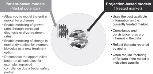
Consider two examples – a patient-based approach and a prescription-based approach, as shown in Figure 3.2. The patient-based modeler starts at the outside of the circle, identifying the number of potential patients with a given disease state, and then ‘contracts’ the potential patients through a series of filters to arrive at those patients who currently are receiving drug therapy. The prescription-based modeler starts with the number of patients currently receiving therapy (that is, currently receiving prescriptions) and then ‘expands’ this number to reach the theoretical maximum. Both approaches yield the same information – it is simply a question of the direction of the analysis.
Figure 3.2 Patient- versus projection-based models
THE PATIENT-BASED ALGORITHM
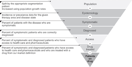
Consider the patient-based algorithm. In this approach we first define the theoretical maximum number of patients with a given disease state and then contract, or filter, the market to arrive at the number of patients who currently are receiving therapy. This is done through a series of filters, as shown in Figure 3.3. The steps involved in filtering from population for a country or region to patients receiving drug therapy are:
• a measure of disease prevalence or incidence;
• an estimate of the number of patients who are symptomatic for the disease;
• an estimate of the number of patients who are diagnosed correctly with the disease;
• an estimate of the number of patients who have access to health care; and
• an estimate of the number of patients who are treated with drug therapy.
This approach has various names in practice – patient filtering, the health care transaction model, patient intervention models, and so forth. Regardless of the name applied, each model determines the difference between the theoretical number of patients and those patients who currently are receiving therapy.
Figure 3.3 Filters used to convert potential patients into treated patients
Epidemiology data – either prevalence or incidence data – are then applied to the population, or relevant population segment, to determine the number of people with a given disease. (An example of this and subsequent calculations in this section are shown in Table 3.1.) The next steps in the algorithm are to estimate how many of these individuals actually express symptoms for the disease and are correctly diagnosed. If these percentages are less than 100 percent, then the potential patient pool subsequently contracts. Note in the example in Table 3.1 that the various filter percentages are changing for the two time points in the illustration. A change in the input assumptions over time is the approach to modeling market growth (or contraction).
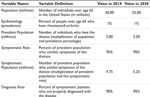
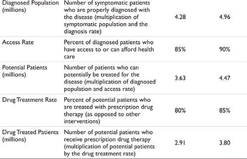
The final filter applied represents the percentage of potential patients (patients with the disease who are symptomatic, correctly diagnosed, and have access to health care) who choose a prescription drug therapy over a non-drug or non-prescription treatment. As discussed earlier, the definition of ‘drug treated’ here is dependent upon the therapy area and the nature of the forecast being requested. Examples include modeling prescription-only treatments, modeling prescription and over-the-counter treatments, modeling alternative medicine, and so forth.
The net result of applying these filters is to convert the population of a given geography into the patients who currently are receiving prescription drug therapy in that same geography. Epidemiology data typically are number less than 100 percent; however, the other filters can approach 100 percent. If this is the case then there is little filtering occurring in the market and the number of patients who receive drug therapy is close to the number of patients with a disease. If, however, any of the filters are at values less than 100 percent this represents growth opportunities in the market. Strategies that increase the flow-through of patients (that is, increase the percentage applied in each of the filters) result in market expansion. We will revisit this concept when we discuss the roles of physician medical education and direct-to-consumer strategies.
THE PRESCRIPTION-BASED ALGORITHM
The above discussion applies to the patient-based forecaster, but what of the person who chooses to model the market potential based on prescription data? This individual effectively starts at the center of the circle in Figure 3.2 and moves to the outside, or to the theoretical maximum. In essence, the forecaster still needs to consider the same filters discussed previously, but the forecaster is looking for the values that allow the current drug-treated patient pool to expand, rather than contract. The only way to expand the market is to identify those variables that can change the universe of currently treated patients and to then grow those variables over time. Once the number of patients with a given disease has been exhausted market expansion must stop – effectively, the forecaster has reached the outer boundary of the circle in Figure 3.2.
COMPARISON OF THE TWO APPROACHES
Which method is preferred? The patient-based forecaster argues that the patient-based method is preferred because it allows the user to identify the theoretical maximum for a product and the pressure points along that way that are constricting the market. The prescription-based forecaster argues that current measures of treatment activity (typical audit data) are more accurate than epidemiology data and that symptomatic and diagnosis rates are difficult to obtain. In essence, the prescription-based forecaster argues that the starting point for the forecast (the data related to current drug usage) is a stronger keystone upon which to build the forecast than the epidemiology data.
Which method is more accurate? Neither, and both. In order to validate the approach both forecasters must use the other method’s data as well. For the patient-based modeler the integrity of the forecast must be ensured by validating the results from the patient flow against actual observations in the market – the audited prescription data. For the prescription-based forecaster the only way to know when to halt the market expansion is to identify the upper boundary of the forecast – essentially the maximum number of patients. Both forecasters require the same information and use the same algorithm – the only difference is the starting point.
EXAMPLES OF SUCCESS AND FAILURE
There are success and failure stories associated with each approach. For the patient-based forecaster success stories revolve around diseases such as benign prostatic hypertrophy and HIV Disease. Benign prostatic hypertrophy (BPH) is a disease that affects men, usually in older age. Cadaveric epidemiological studies suggested that the prevalence of BPH was as high as 95 percent in men over the age of 65. However, the number of men treated for BPH was significantly lower. With the advent of new diagnostic technologies, physicians were able to monitor for an enzyme associated with BPH and were able to diagnose patients earlier in their disease. This led to market growth through an increase in diagnosis rates.
A similar story is associated with HIV disease. With the appearance of new diagnostic tools for the HIV virus (specifically the enhanced sensitivity of PCR-based diagnostic tools) patients with lower levels of the HIV virus were identified earlier and were placed on anti-HIV medications. Again, the use of diagnostic tools enabled market expansion.
Changes in the rate of symptom recognition also increase the size of the market. Examples here include self-examination for breast and testicular cancers, education about transient ischemic events that may lead to stroke, and recognition that persistent heartburn may be a symptom of other gastrointestinal disorders.
Although the discussion above has been restricted to two examples – patient-based and prescription-based models – similar logic applies to the use of other databases, such as days of therapy, cycles of treatment, and so forth. For acute disease states where there may be multiple treatment opportunities in a single year the forecast may be modeled using ‘treatment episodes’ instead of patients. An example of this would be a forecast for migraine headache, where each patient may experience multiple migraines in a given year. Each episode represents an opportunity for treatment and must therefore be captured explicitly in the forecast model.
PREVALENCE VERSUS INCIDENCE MODELS
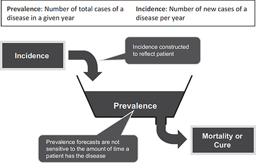
There are two approaches for modeling the epidemiology associated with diseases: prevalence and incidence. These two methods are illustrated in Figure 3.4. In a prevalence-based model the user is concerned with the total number of cases of a disease in a given year. Patient history is not needed. It doesn’t matter if the patient is in their first, tenth, or fifteenth year having the disease because the treatment options do not vary significantly.
In an incidence-based epidemiology model patient history is critical. The choice of drug treatment options is related to patient history – a ‘naïve’ patient who has just been diagnosed with the disease is treated differently than a patient who has prior treatment experience. If the patient is near the end of their treatment cycle – either through cure, remission, or mortality – the choice of treatment options may also differ. If a patient progresses through stages of a disease then an incidence-based platform may need to be used. If the choice of treatment regimen in a latter stage of the disease is dependent upon the drugs used in an earlier stage, the forecaster must use an incidence-based model.
Figure 3.4 Prevalence- and incidence-based epidemiology
Both types of model are used in forecasting, but prevalence-based platforms are simpler to construct and to use. This is because of the ‘accounting’ necessary in incidence-based models. The need to keep track of patients on an annual basis and the treatment history associated with each patient cohort adds complexity to the forecast model. For example, consider a forecast over a five-year period for a disease that has two stages. During year five of the forecast model there are ten patient cohorts that need to be accounted for separately, each with potentially different competitive environments, drugs, compliance rates, mortality rates, and so forth. Conversely, in a prevalence-based model there would be a maximum of two cohorts – one for each disease stage. In a multi-year, multistage disease the complexity of the forecast model can be significant.
When needed, however, incidence-based models can be created. Simple incidence-based models can be constructed in spreadsheet software such as Microsoft Excel. For complex models there exists a set of ‘systems dynamics’ software packages that can be used. Several therapy areas require incidence-based models: oncology, transplantation, and HIV disease. This requirement occurs because the drug treatment regimen in these disease areas change as a patient progresses through the disease state or treatment options. The choice of subsequent therapies may be dependent upon a patient’s response to prior therapy. Both the central nervous system and cardiovascular disease states increasingly are modeled using incidence-based approaches as pharmaceutical companies attempt to model out patient flow at a more detailed level.
PATIENT-BASED VERSUS PATIENT-FLOW MODELS
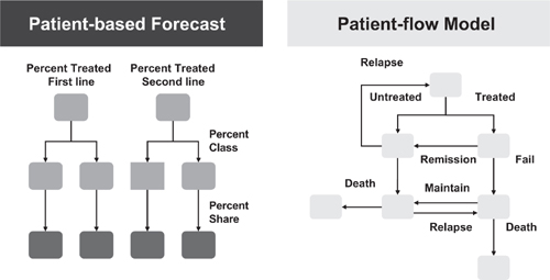
Figure 3.5 provides an overview of patient-based versus patient-flow models. Patient-based models are best suited for markets where patients can be allocated to different ‘buckets’ of treatment paradigms, and there is no interdependency between the choice of therapy and progression of disease. Patient-flow models are more dynamic, capturing the time dependencies between patient progression in a given disease state and interdependencies between treatment options. If patients can be allocated to treatment buckets via a simple decision tree analysis, patient-based modeling is appropriate. If, however, patients may cycle between treatment groups, and the choice of therapy may be dependent upon prior treatment history, patient-flow models are most applicable.
Figure 3.5 Patient-based and patient-flow models
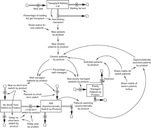
Figure 3.6 An example of a systems dynamics forecast model
Construction of patient-flow models is not possible in linear thinking programs such as Excel. In attempting to construct patient-flow models using spreadsheet software the user will receive ‘circular reference’ errors due to the circular loops encountered in modeling patient movement between disease states or treatment options. Patient-flow models are constructed best in systems dynamics software programs such as iThink, Vensim, or Powersim. An example of a forecast model constructed using a systems dynamics approach is shown in Figure 3.6. (Note that this is a purely illustrative example; readers who wish to pursue patient flow models in more detail are referred to the book by Paich et al. listed in the References.) The interdependence of treatment options and time-dependence of patient flows in incidence-based therapy areas makes systems dynamics the software of choice when an incidence-based forecast model is required.
PATIENT SEGMENTATION
The approach discussed to date for modeling the market for a product has assumed an undifferentiated patient pool – that is, potential segments of patients have been treated the same in the forecast algorithm. Often this is not a valid assumption and the forecaster needs to divide the patient pool into relevant segments. Examples of common segmentation patterns might be by age, by gender, by race, by severity of the disease, by stage of the disease, and so forth. Less common – but just as valid – examples of patient segmentation include: by specialty of the physician who treats the patient, by treatment site, by risk-factors, or by geography. There are no absolutes in selecting an appropriate segmentation pattern; however, the choice of the segments to forecast should be aligned to the questions and strategies that need to be addressed using the forecast model.
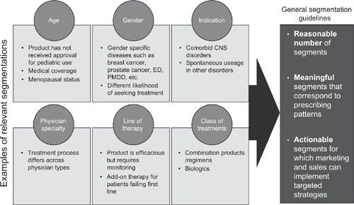
Once a segmentation pattern is selected the market component of the forecast algorithm (Figure 3.1) must be modified according to the segmentation pattern. For example, if the patients are segmented into three age cohorts, the population used in the forecast flow must also be segmented into the three age cohorts. Several examples of segmentation patterns are shown in Figure 3.7 along with general segmentation guidelines.
The segmentation can be preserved throughout the forecast flow or the segments can be combined at any point in the forecast algorithm. The decision to hold the segmentation pattern throughout the forecast or to combine segments at various points should be reflective of the market dynamics as well as the purpose for the forecast. Given the number of potential segmentation variables and the number of points of expansion and collapse of segments in the forecast algorithm, it is easy to envision an almost unlimited set of possibilities for the patient flow. One of the biggest challenges to the forecaster is to decide on the appropriate segmentation pattern. Since this is an ‘upstream’ decision that affects many of the ‘downstream’ variables the choice of segmentation becomes a critical factor in forecast model design.
Figure 3.7 Examples of patient segmentation
The forecaster must be careful not to be seduced by the lure of too many segments in the forecast model. What can be a very satisfying academic exercise in creating segments for subpopulations in a therapy area often turns into a frustrating exercise of collecting data for very targeted (and small) segments. It is not unusual for a forecaster to create a finely segmented forecast algorithm, only to have to collapse many of the segments when the data are not available for the desired segmentation.
MODELING ‘CONSUMER EDUCATION’ EFFECTS ON THE MARKET
Recent years have seen the advent of increasing ‘consumer education’ efforts, either through the information dissemination by advocacy groups using tools such as the Internet or through direct-to-consumer advertising campaigns in markets such as the United States. The effects of such educational efforts are multifold – affecting variables in all three sections of the new product forecast algorithm (see Figure 3.1). In this section we examine the effects of consumer education in the market.
Figure 3.8 The effects of consumer education and direct-to-consumer marketing
Consumer education and direct-to-consumer advertising can be modeled using three variables that affect assumptions in the forecast model. These three variables are consumer awareness, consumer intent, and consumer action (see Figure 3.8). Consumer awareness acts upon the ability of a patient (and physician) to recognize the symptoms and correctly diagnose a given disease. In theory, educating the patient allows for better self-recognition of disease symptoms and diagnosis (or at least creating awareness that a physician visit for a diagnosis is required). This dynamic – coupled with educating the patient that a drug-therapy is available – is captured in a change in consumer awareness and is translated into increased percentages of symptom recognition and self-diagnosis. In essence, raising the consumer awareness variable increases the market size. The implicit assumption behind product-specific consumer education programs (that is, direct-to-consumer advertising campaigns) is that this increase in market size will be followed by a direct increase in prescribing behavior for the product being discussed. We will revisit this assumption when discussing product share projections.
There are, however, mitigating variables to increased consumer awareness. The dynamics of consumer intent and consumer action (willingness to act upon that intent) govern changes in the percentage of patients who are treated with drug therapy. Once the consumer is aware of a given disease state they must then visit their physician or health-care provider before a drug can be prescribed. This action of intent to visit a physician, and actual willingness to act upon that intent, govern the changes in the percentage of patients who will receive drug therapy as a result of their heightened awareness. In a perfect scenario, 100 percent of all consumers who are aware of drug therapy options would visit their physician and receive a prescription. However, in the absence of perfect behavior (a realistic assumption) the consumer intent and willingness to act upon that intent variables are less than 100 percent.
Estimating consumer intent and willingness to act upon that intent are significant challenges for the forecaster. There are many well-developed and documented methodologies for measuring consumer awareness, and all of the reputable vendors who perform consumer education and direct-to-consumer advertising campaigns will have historical data that measure the change in consumer awareness. In the case of direct-to-consumer advertising campaigns these measurements are available for all types of advertising media – print, radio, television – and across many types of consumer demographics.
Stay updated, free articles. Join our Telegram channel

Full access? Get Clinical Tree


