and Philip Yip1
(1)
The Photophysics Research Group, Department of Physics, Centre for Molecular Nanometrology, SUPA, University of Strathclyde, Glasgow, Scotland, UK
Abstract
Methods and protocols are described when using fluorescence metrology to determine the average nanoparticle (np) size in colloids in the range of 1–10 nm. The technique is based on determining the rotational correlation time of the np from the decay of fluorescence anisotropy of a dye that is electrostatically or covalently attached to the np as it undergoes Brownian rotation. The np size is then calculated from the Stokes–Einstein equation. The exemplar of silica nps is presented, but the approach can also be applied to other types of nps.
Key words
Fluorescence anisotropy decayFluorescence lifetimeNanoparticleSilicaNanometrologyLUDOX® Sol–gelTCSPC1 Introduction
Measurement science on the nanoscale (nanometrology) is widely seen as a key to progress in the many burgeoning applications of nanotechnology. These applications span not only science and technology but also engineering and medicine. Global interest in the metrology of nanoparticles (nps) in particular has undergone quite a renaissance in recent times. This is because of the development of novel manifestations of nps such as carbon nanotubes, noble metal, diamond, and semiconductor quantum dots. Irrespective of physical and chemical differences between nps, there is a certain common concern in respect of the potential toxicological and environmental issues surrounding not only new types of nps but also older structures. Carbon nps from combustion and metal oxide nps such as silica and titania are some of the latter that immediately spring to mind. As a paradigm here we consider only silica. Also, we confine ourselves to the 1–10 nm np range as this is where there is a particularly urgent need for globally accepted standards and precise measurement techniques. Such small nps are known to traverse cellular membranes with ease, are at the limit of present-day measurement techniques, and yet are most appropriate for study in a colloid using fluorescence nanometrology. Traditional methods for nanoparticle metrology, such as small angle X-ray and neutron scattering, are much more expensive, complex, and difficult to use when compared to fluorescence nanometrology, as we will describe here.
Fluorescence nanometrology can be defined as the use of fluorescence to determine nanoscale lengths. When it comes to tracking rapidly changing phenomena involving nps on the scale of super-molecular dimensions, fluorescence decay time techniques have few equals [1]. This is because they can be performed in situ, have an appropriate timescale (ps to ns), offer high sensitivity (down to the single-molecule, single-photon level), and benefit from the wide range of well-characterized fluorescence probes with which to customize a study. The associated equipment is also now extremely easy to use, reliable, and relatively inexpensive. However, the interpretation of data still benefits from skill and experience. Here, we describe the use of the decay of fluorescence anisotropy to determine np size.
The measurement approach is depicted in Fig. 1 for the case of dye molecules partitioned between dual Brownian motions relating to when bound to a np and when rotating freely.
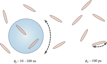
Fig. 1
Depicts a dye rotating free (ϕ d ~ 100 ps) and rotating bound to a nanoparticle (ϕ p ~ 10–100 ns) in a colloid
The rotational correlation time of the free dye of known radius gives the local viscosity of the solution using the Stokes–Einstein equation. When the viscosity is combined in the same equation with the rotational correlation time of the dye bound to nps this leads to determination of the np radius. Both stable [2] and changing [3] np sizes can in principle be measured (see Note 1).
2 Materials: Chemical Preparation
As fluorescence is an extremely sensitive technique, we stress that all glassware must be sufficiently cleaned before use (see Notes 2 and 3). Prepare and store all reagents at room temperature (unless indicated otherwise). Use distilled water (unless indicated otherwise). Cap all chemicals and create an additional seal with parafilm (unless indicated otherwise). Label each chemical/sample being used (see Note 4) and preferably store in the dark. Diligently follow all waste disposal regulations when disposing of waste chemicals.
2.1 Stöber Synthesis of Silica Nanoparticles
The Stöber process is the ammonia-catalyzed reaction of an orthosilicate, e.g., tetraethyl orthosilicate (TEOS: Si(OR)4; R=C2H5) with water in low molecular weight alcohols to produce monodispersed, spherical silica nanoparticles (see Fig. 2). This method, as specified by Green et. al. [4], produces a narrow size distribution of spherical particles as in the case of LUDOX®.
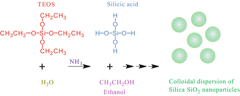
Fig. 2
Schematic of the Stöber synthesis of nps
1.
10 ml sols will be produced using a conical flask.
2.
3.
We recommend making a tertiary diagram like our Fig. 3. From this, calculate the ratio of ammonia, water, and TEOS for the desired sample. For accuracy, we recommend calculating the mass of each component you will require for your sample (see Note 7).
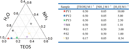
Fig. 3
Ternary diagram of colloidal silica compositions
4.
Make a water–ammonia solution of desired concentration. This solution should be made in a separate glass container which is placed on a balance and zeroed. The water should be first added by using a pipette. The 33 % ammonia solution should be quickly added to the water using a Pasteur pipette. The container should be immediately capped and shaken to ensure that it has completely mixed (see Note 8).
5.
Place the 10 ml conical flask on the balance and zero it. Add the desired volume of TEOS using a Pasteur pipette.
7.
Next, add the water–ammonia solution and fill up to the 10 ml mark using methanol.
9.
Place the conical flask on a magnetic stirrer for 24 h at a gentle setting.
2.2 Fluorescent Dye Preparation
Like all fluorescence measurements, an appropriate dye must be selected. The dye must meet two criteria: first, it must attach to the np under investigation and second have appropriate photophysical properties (e.g., fluorescence decay) for tracking the np rotation. For anisotropy measurements of nanoparticles, the dye may attach to the system electrostatically or covalently. Before working with a new dye, it is important to record the steady-state absorption and emission spectra so one has a basic understanding of the photophysical properties of the dye. We will take rhodamine 6G as an example here.
1.
3.
Record a steady-state absorption spectrum like that of Fig. 4 using a spectrophotometer (see Note 18). In our case, we used a Jasco V660 spectrophotometer. A second identical, and preferably matched, cuvette filled with only the pure solvent should be used in the reference channel.
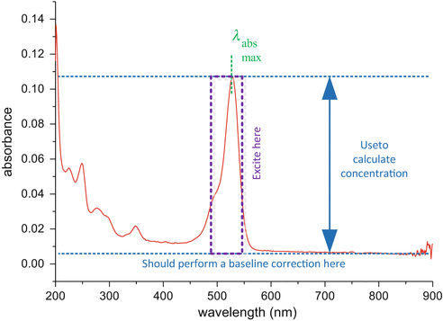
Fig. 4
Absorption spectra of rhodamine 6G in methanol. In this example the path length was 10 cm and therefore the concentration in the cuvette is ~ 0.1 μM. One can clearly see the most suitable wavelength region for excitation
4.
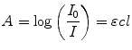
From the absorption spectra you can verify the dye concentration in the cuvette using the Beer–Lambert law Eq. 1 (see Note 19)
(1)
where  is the absorbance,
  and
and  are the intensity of the incident and transmitted light, respectively,
  is the concentration in
  ,
,  is the path length in cm, and
  is the molar extinction coefficient in
  .
.
is the absorbance, and are the intensity of the incident and transmitted light, respectively, is the concentration in , is the path length in cm, and is the molar extinction coefficient in .5.
6.
From the absorption spectra, select a suitable pulsed light source for excitation. This should have a peak wavelength in a region where the dye has a high absorbance. In our case, we selected an IBH 503 nm DeltaDiode.
7.
Record a steady-state emission spectrum using a spectrofluorometer and select the excitation wavelength to match that of your selected light source (see Note 22). In our case, we used a HORIBA Fluorolog 3 spectrophotometer.
8.
Normalize and overlay both absorption and emission spectra as our Fig. 5.
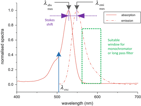
Fig. 5
Normalized absorption and emission spectra of rhodamine 6G, excited at 503 nm. From this one can calculate the Stokes shift and see what wavelength range is the best for measuring the fluorescence
9.
Measure the Stokes shift and select an appropriate long-pass filter or monochromator wavelength for later use with lifetime measurements (see Note 23).
2.2.1 Electrostatic Labelling
Due to electrostatic interactions, cationic dyes will readily bind to negatively charged silica colloids in alkaline solution (see Note 24) and vice versa.
1.
Measure the pH of the colloid.
2.
Prepare an oppositely charged dye that will affix to the np by electrostatic interaction.
3.
In this case, rhodamine 6G as prepared above will be used as an example.
4.
6.
Prepare a similar dye that does not bind to the np, for example, Rhodamine B, in exactly the same manner as rhodamine 6G.
7.
A dye such as Rhodamine B that does not bind to the np can be used to determine the microviscosity. We recommend preparing both dyes for a comparison. See Fig. 6 for the chemical structures of both dyes.
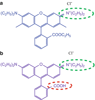
Fig. 6
Chemical structure of (a) rhodamine 6G and (b) rhodamine B. Note the electrostatic attraction circled green for both dyes and the electrostatic repulsion from the carboxylic acid group circled red for rhodamine B
2.2.2 Covalent Labelling
For covalent labelling, a dye needs to not only be selected with appropriate properties as listed previously but must also possess chemical linkers for binding to the np [5]. In this example, Fluorescein 5(6)-isothiocyanate (FITC) will be bound to 3-aminopropyl trimethoxysilane (APS). Such a labelling approach has previously been used with silica nanoparticles [6–8]. See Fig. 7 for chemical structures and the reaction mechanism.
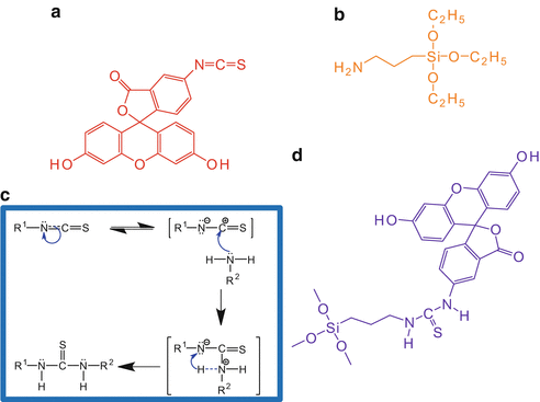
Fig. 7
(a) Fluorescein 5(6)-isothiocyanate (FITC) is bound to (b) 3-aminopropyl trimethoxysilane (APS) via the mechanism (c) to create (d) FITC–APS
4.
Seal and stir at room temperature at a high speed for 30 min.
6.
Dry the top of the vial with Nitrogen.
7.
Seal and stir at a high speed at room temperature for ~24–72 h.
2.3 Adding the Dye to the Nanoparticle
4.
Measure the emission spectra, excited by the appropriate wavelength from the light source.
2.4 Preparation of a Scattering Colloid for Recording the Excitation Pulse
1.
Add 17 ml of water to a 30 ml glass vial.
2.
Add 2 ml of 0.1 M sodium hydroxide.
3.
Add 1 ml of LUDOX SM30.
4.
5.
The scatter colloid is quite stable if left sealed, but we recommend replacing it every month (see Note 28).
3 Methods: Decay Time Techniques
3.1 Acquisition of Data
It is generally accepted that anisotropy decay time measurements are best performed in the time domain using time-correlated single-photon counting techniques (TCSPC) [9, 10]. A schematic of such a fluorometer is shown in Fig. 8. In our case, we have used a FluoroCube from Horiba Jobin Yvon IBH Ltd, Glasgow.
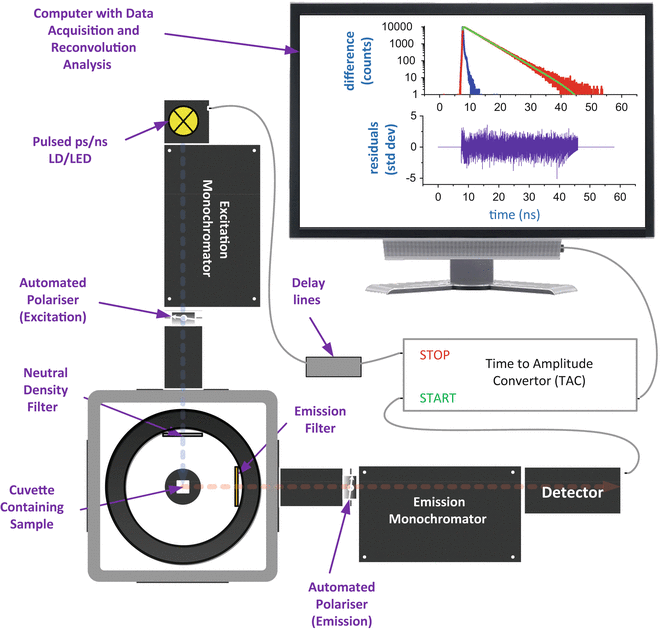
Fig. 8
Schematic of the fluorometer used for fluorescence anisotropy decay measurements. Fluorescence photons are detected using a single-photon timing detection system. Fluorescence decay data are accumulated using the FluoroHub electronics which incorporate a time-to-amplitude converter (TAC), operated in reverse mode to minimize dead time, and multichannel analyzer. The operation of all functions is fully controlled under Microsoft Windows software
3.1.1 Fluorescence Decay Time Measurement
The fluorescence lifetime is the average time a fluorescent dye remains in an excited state before emission of a photon (see Notes 29 and 30).
1.
2.
Choose a suitable detector with a compatible wavelength response and single-photon timing sensitivity for your sample. In our case, a compact photomultiplier in a T0-8 package (Hamamatsu Model R7400) (see Note 32).
3.


Ensure the light source and the detector are at right angles to each other in l-format orientation (see Fig. 8 and Note 33).
Stay updated, free articles. Join our Telegram channel
Full access? Get Clinical Tree
