Multistrain Disease Dynamics


(1)
Department of Mathematics, University of Florida, Gainesville, FL, USA


8.1 Competitive Exclusion Principle


The causative agents of diseases, such as viruses and bacteria, may be represented by multiple variants, called by the general name strains (or subtypes). The presence of multiple strains of a pathogen complicates our ability to combat the disease. For instance, in influenza, it is believed that each strain imparts permanent immunity, but drift evolution creates new strains, and in a new flu season, we can contract the disease again. There are other diseases whose causative agents are represented by multistrain pathogens. For example, Haemophilus influenzae, which is responsible for a range of infections, is represented by six serotypes: a, b, c, d, e, and f, as well as some variants that are not typeable. Streptococcus pneumonae is represented by 90 serotypes. Dengue virus has four serotypes. In this chapter, we study models with multiple strains.

In ecology, the competitive exclusion principle is one of the main principles that govern species competition. The principle was first formulated as a law in the 1930s by the Russian ecologist Georgy Gause [64], who discovered it based on laboratory experiments. In short, the principle can be stated as complete competitors cannot coexist. In this section, we introduce through models the epidemiological context of this principle.


8.1.1 A Two-Strain Epidemic SIR Model


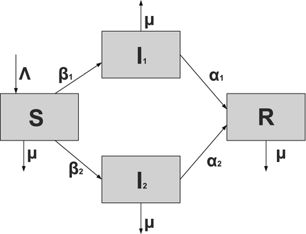
To account for the genetic variability of the pathogen, we investigate an SIR epidemic model with multiple strains. The the two-strain model has the following compartments: S(t) is the number of susceptible individuals at time t, I 1(t) is the number of individuals infected by strain one, I 2(t) is the number of individuals infected by strain two, and R(t) is the number of recovered individuals. We assume that each strain, once contracted, imparts permanent immunity to itself and to the other strain.

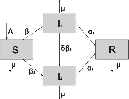
Susceptible individuals can become infected either by strain one at a transmission rate β 1 or by strain two at a transmission rate β 2. Those infected with strain one recover at a rate α 1, and those infected with strain two recover at a rate α 2. Susceptible individuals are recruited at a rate Λ. Individuals in all classes die at a natural death rate μ. The model is given below. The flowchart of the model is given in Fig. 8.1:
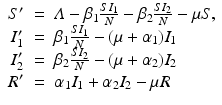


$$\displaystyle\begin{array}{rcl} S'& =& \varLambda -\beta _{1}\frac{SI_{1}} {N} -\beta _{2}\frac{SI_{2}} {N} -\mu S, \\ I_{1}'& =& \beta _{1}\frac{SI_{1}} {N} - (\mu +\alpha _{1})I_{1} \\ I_{2}'& =& \beta _{2}\frac{SI_{2}} {N} - (\mu +\alpha _{2})I_{2} \\ R'& =& \alpha _{1}I_{1} +\alpha _{2}I_{2} -\mu R {}\end{array}$$

(8.1)
The total population size N is given by 
$$N(t) = S(t) + I_{1}(t) + I_{2}(t) + R(t)$$
. Adding the equations above, we see that the equation of the total population size is the simplified logistic 
$$N'(t) =\varLambda -\mu N$$
.

A304573_1_En_8_Fig1_HTML.gif


Fig. 8.1
A flowchart of an SIR model with two strains and perfect immunity

The next step will be to compute the equilibria. Working with a standard incidence allows us to consider the equilibrium equations of the proportions. For the equilibrial values of the variables S, I 1, I 2, and R, we set 
$$s = S/N$$
, 
$$i_{1} = I_{1}/N$$
, 
$$i_{2} = I_{2}/N$$
, 
$$r = R/N$$
. Since N satisfies the equation 
$$0 =\varLambda -\mu N$$
, and hence Λ = μ N, the equations for the equilibrium proportions are given by
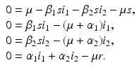


$$\displaystyle{ \begin{array}{l} 0 =\mu -\beta _{1}si_{1} -\beta _{2}si_{2} -\mu s, \\ 0 =\beta _{1}si_{1} - (\mu +\alpha _{1})i_{1}, \\ 0 =\beta _{2}si_{2} - (\mu +\alpha _{2})i_{2}, \\ 0 =\alpha _{1}i_{1} +\alpha _{2}i_{2} -\mu r.\end{array} }$$

(8.2)
Model (8.1) has three equilibria. The model has a disease-free equilibrium in which neither strain one nor strain two is present. At the disease-free equilibrium, we have 
$$s = 1,i_{1} = 0,i_{2} = 0,r = 0$$
. Hence, the disease-free equilibrium in the original variables is given by 
$$\mathcal{E}_{0} = \left (\frac{\varLambda }{\mu },0,0,0\right )$$
. In contrast to single-strain models, multistrain models have multiple reproduction numbers, one for each strain. To define the reproduction numbers associated with strain one and strain two, we have to look at the local stability of the disease-free equilibrium. Computing the Jacobian at the disease-free equilibrium yields


$$\displaystyle{ J = \left (\begin{array}{cccc} -\mu & \qquad -\beta _{1} & \qquad -\beta _{2} & \qquad 0 \\ 0 &\qquad \beta _{1} - (\mu +\alpha _{1})& \qquad 0 & \qquad 0 \\ 0 & \qquad 0 &\qquad \beta _{2} - (\mu +\alpha _{2})& \qquad 0 \\ 0 & \qquad \alpha _{1} & \qquad \alpha _{2} & \qquad -\mu \end{array} \right ). }$$

(8.3)
The characteristic equation 
$$\vert J -\lambda I\vert = 0$$
has one double eigenvalue 
$$\lambda _{1} =\lambda _{2} = -\mu$$
, and the following two eigenvalues:


$$\displaystyle\begin{array}{rcl} \lambda _{3}& =& \beta _{1} - (\mu +\alpha _{1}), \\ \lambda _{4}& =& \beta _{2} - (\mu +\alpha _{2}).{}\end{array}$$

(8.4)
The disease-free equilibrium is locally asymptotically stable if λ 3 < 0 and λ 4 < 0. We notice that the eigenvalue λ 3 is associated with strain one and gives rise to the reproduction number of strain one, 
$$\mathcal{R}_{1}$$
. The eigenvalue λ 4 is associated with strain two and gives rise to the reproduction number of strain two, 
$$\mathcal{R}_{2}$$
. Thus, we define


$$\displaystyle{ \mathcal{R}_{1} = \frac{\beta _{1}} {\mu +\alpha _{1}},\qquad \qquad \mathcal{R}_{2} = \frac{\beta _{2}} {\mu +\alpha _{2}}. }$$

(8.5)
We have the following result:


Proposition 8.1.

The disease-free equilibrium of system (8.1) is locally asymptotically stable if both reproduction numbers are less than 1, that is if


$$\displaystyle{\mathcal{R}_{1} < 1\qquad \qquad \mathcal{R}_{2} < 1.}$$
The disease-free equilibrium is unstable if at least one of the above inequalities is reversed.


8.1.2 The Strain-One- and Strain-Two-Dominance Equilibria and Their Stability


A strain-one-dominance equilibrium is a boundary equilibrium in which strain one is present i 1 ≠ 0, while strain two is not present i 2 = 0. From the second equation in (8.2), we have


$$\displaystyle{s = \frac{\mu +\alpha _{1}} {\beta _{1}} = \frac{1} {\mathcal{R}_{1}}.}$$
We need s < 1 for it to be a proper fraction. Thus, for a strain-one-dominance equilibrium to be meaningful, we need 
$$\mathcal{R}_{1} > 1$$
” src=”/wp-content/uploads/2016/11/A304573_1_En_8_Chapter_IEq14.gif”></SPAN>. To compute the value of the infected individuals with strain one, we start from the first equation:<br />
<DIV id=Equc class=Equation><br />
<DIV class=EquationContent><br />
<DIV class=MediaObject><IMG alt=
Replacing s with 
$$1/\mathcal{R}_{1}$$
and solving for i 1, we have


$$\displaystyle\begin{array}{rcl} i_{1}& =& \frac{\mu } {(\mu +\alpha _{1})\mathcal{R}_{1}} = \frac{\mu } {\mu +\alpha _{1}}\left (1 - \frac{1} {\mathcal{R}_{1}}\right ), \\ r& =& \frac{\alpha _{1}} {\mu } i_{1} = \frac{\alpha _{1}} {\mu +\alpha _{1}}\left (1 - \frac{1} {\mathcal{R}_{1}}\right ). {}\end{array}$$

(8.6)
The strain-one-dominance equilibrium is given by


$$\displaystyle{\mathcal{E}_{1} = \left ( \frac{1} {\mathcal{R}_{1}} \frac{\varLambda } {\mu }, \frac{\mu } {\mu +\alpha _{1}}\left (1 - \frac{1} {\mathcal{R}_{1}}\right )\frac{\varLambda } {\mu },0, \frac{\alpha _{1}} {\mu +\alpha _{1}}\left (1 - \frac{1} {\mathcal{R}_{1}}\right )\frac{\varLambda } {\mu }\right ).}$$
A strain-two-dominance equilibrium is a boundary equilibrium in which strain two is present i 2 ≠ 0, while strain one is not present i 1 = 0. A strain-two-dominance equilibrium exists if and only if 
$$\mathcal{R}_{2} > 1$$
” src=”/wp-content/uploads/2016/11/A304573_1_En_8_Chapter_IEq16.gif”></SPAN>. The strain-two-dominance equilibrium is given by<br />
<DIV id=Eque class=Equation><br />
<DIV class=EquationContent><br />
<DIV class=MediaObject><IMG alt=

An equilibrium for which both strain one and strain two are present, that is, i 1 ≠ 0 and i 2 ≠ 0, is called a coexistence equilibrium. The equilibrium value of s in a coexistence equilibrium satisfies the following two equations, which are obtained from (8.2):


$$\displaystyle\begin{array}{rcl} 0& =& \beta _{1}s - (\mu +\alpha _{1}), \\ 0& =& \beta _{2}s - (\mu +\alpha _{2}).{}\end{array}$$

(8.7)
The first equation requires


$$\displaystyle{s = \frac{\mu +\alpha _{1}} {\beta _{1}} = \frac{1} {\mathcal{R}_{1}}.}$$
The second equation requires


$$\displaystyle{s = \frac{\mu +\alpha _{2}} {\beta _{2}} = \frac{1} {\mathcal{R}_{2}}.}$$
These two expressions for s can be consistent if and only if 
$$\mathcal{R}_{1} = \mathcal{R}_{2}$$
. Hence, in the generic case in which the two strains have different reproduction numbers, a coexistence equilibrium does not exist.

To investigate the stability of the dominance equilibria, we consider the Jacobian at an equilibrium 
$$\mathcal{E} = (s,i_{1},i_{2},r)$$
. Because N(t) is asymptotically constant, we treat it as constant. It can be checked that this does not change the results.


$$\displaystyle{ J = \left (\begin{array}{cccc} -\beta _{1}i_{1} -\beta _{2}i_{2}-\mu & \qquad -\beta _{1}s & \qquad -\beta _{2}s & \qquad 0 \\ \beta _{1}i_{1} & \qquad \beta _{1}s - (\mu +\alpha _{1})& \qquad 0 & \qquad 0 \\ \beta _{2}i_{2} & \qquad 0 &\qquad \beta _{2}s - (\mu +\alpha _{2})& \qquad 0 \\ 0 & \qquad \alpha _{1} & \qquad \alpha _{2} & \qquad -\mu \end{array} \right ). }$$

(8.8)
To determine the local stability of a strain-one-dominance equilibrium, we consider the Jacobian at that equilibrium:


$$\displaystyle{ J(s,i_{1},0,r) = \left (\begin{array}{cccc} -\beta _{1}i_{1}-\mu & \qquad -\beta _{1}s & \qquad -\beta _{2}s & \qquad 0 \\ \beta _{1}i_{1} & \qquad \beta _{1}s - (\mu +\alpha _{1})& \qquad 0 & \qquad 0 \\ 0 & \qquad 0 &\qquad \beta _{2}s - (\mu +\alpha _{2})& \qquad 0 \\ 0 & \qquad \alpha _{1} & \qquad \alpha _{2} & \qquad -\mu \end{array} \right ). }$$

(8.9)
The Jacobian has one eigenvalue 
$$\lambda _{1} = -\mu$$
, and another


$$\displaystyle{\lambda _{2} =\beta _{2}s - (\mu +\alpha _{2}) = (\mu +\alpha _{2})\left (\frac{\mathcal{R}_{2}} {\mathcal{R}_{1}} - 1\right ).}$$
The eigenvalue λ 2 is called the growth rate of strain two when strain one is at equilibrium. The remaining eigenvalues of the strain-one-dominance equilibrium are the eigenvalues of the 2 × 2 matrix


$$\displaystyle{ \left (\begin{array}{cc} -\beta _{1}i_{1}-\mu & \qquad -\beta _{1}s \\ \beta _{1}i_{1} & \qquad \beta _{1}s - (\mu +\alpha _{1})\\ \end{array} \right ). }$$

(8.10)

We notice that the entry in the second row, second column in the matrix above is 
$$\beta _{1}s - (\mu +\alpha _{1}) = 0$$
, since 
$$s = 1/\mathcal{R}_{1}$$
. Hence, the above matrix has Tr = 
$$-\beta _{1}i_{1}-\mu < 0$$
and Det = β 1 s β 1 i 1 > 0. Thus, the eigenvalues of the above matrix are negative or have negative real part. We conclude that the local stability of the dominance equilibrium 
$$\mathcal{E}_{1}$$
depends on the sign of the eigenvalue λ 2. A dominance equilibrium 
$$\mathcal{E}_{1}$$
is locally asymptotically stable if and only if λ 2 < 0. Consequently, the dominance equilibrium 
$$\mathcal{E}_{1}$$
is locally asymptotically stable if and only if 
$$\mathcal{R}_{2} < \mathcal{R}_{1}$$
, that is, when strain one has a larger reproduction number than strain two. By symmetry, a dominance equilibrium 
$$\mathcal{E}_{2}$$
is locally asymptotically stable if and only if 
$$\mathcal{R}_{2} > \mathcal{R}_{1}$$
” src=”/wp-content/uploads/2016/11/A304573_1_En_8_Chapter_IEq28.gif”></SPAN>, that is, when strain two has a larger reproduction number than strain one. We summarize these results in the following theorem:</DIV><br />
<DIV id=FPar2 class=
Theorem 8.1.

A strain-j-dominance equilibrium exists if and only if 
$$\mathcal{R}_{j} > 1$$
” src=”/wp-content/uploads/2016/11/A304573_1_En_8_Chapter_IEq29.gif”></SPAN> <SPAN class=EmphasisTypeItalic>. If</SPAN> <SPAN id=IEq30 class=InlineEquation><IMG alt= \mathcal{R}_{2}$$ ” src=”/wp-content/uploads/2016/11/A304573_1_En_8_Chapter_IEq30.gif”> , then the strain-one-dominance equilibrium is locally asymptotically stable. If 
$$\mathcal{R}_{1} < \mathcal{R}_{2}$$
, it is unstable. If 
$$\mathcal{R}_{1} < \mathcal{R}_{2}$$
, then the strain-two-dominance equilibrium is locally asymptotically stable. If 
$$\mathcal{R}_{1} > \mathcal{R}_{2}$$
” src=”/wp-content/uploads/2016/11/A304573_1_En_8_Chapter_IEq33.gif”></SPAN> <SPAN class=EmphasisTypeItalic>, it is unstable. Coexistence is not possible outside of the degenerate case</SPAN> <SPAN id=IEq34 class=InlineEquation><IMG alt= .

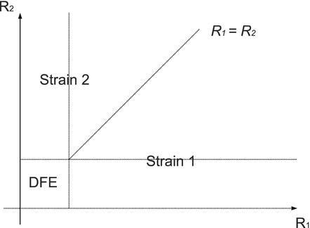
Figure 8.2 gives the competitive outcomes for the two strains. The competitive outcomes are also listed in Table 8.1.

A304573_1_En_8_Fig2_HTML.gif


Fig. 8.2
Strain-one and strain-two dominance regions. The 45 line is the line 
$$\mathcal{R}_{1} = \mathcal{R}_{2}$$
. Above that line is the region 
$$\mathcal{R}_{2} > \mathcal{R}_{1}$$
” src=”/wp-content/uploads/2016/11/A304573_1_En_8_Chapter_IEq48.gif”></SPAN>, where strain two outcompetes strain one. Below this line is the region <SPAN id=IEq49 class=InlineEquation><IMG alt=, where strain one outcompetes strain two


Table 8.1
Competitive outcomes for the two-strain model (8.1)


Region

Long-term behavior

Competitive outcome


$$\mathcal{R}_{1} < 1$$
, 
$$\mathcal{R}_{2} < 1$$

I 1(t) → 0, I 2(t) → 0

Both strains die out


$$\mathcal{R}_{1} > 1$$
” src=”/wp-content/uploads/2016/11/A304573_1_En_8_Chapter_IEq37.gif”></SPAN>, <SPAN id=IEq38 class=InlineEquation><IMG alt=

I 1(t) persists, I 2(t) → 0

Strain 1 dominates


$$\mathcal{R}_{1} < 1$$
, 
$$\mathcal{R}_{2} > 1$$
” src=”/wp-content/uploads/2016/11/A304573_1_En_8_Chapter_IEq40.gif”></SPAN> </DIV></TD><br />
<TD><br />
<DIV class=SimplePara><SPAN class=EmphasisTypeItalic>I</SPAN> <SUB>1</SUB>(<SPAN class=EmphasisTypeItalic>t</SPAN>) → 0, <SPAN class=EmphasisTypeItalic>I</SPAN> <SUB>2</SUB>(<SPAN class=EmphasisTypeItalic>t</SPAN>) persists</DIV></TD><br />
<TD><br />
<DIV class=SimplePara>Strain 2 dominates</DIV></TD></TR><br />
<TR class=noclass><br />
<TD><br />
<DIV class=SimplePara><SPAN id=IEq41 class=InlineEquation><IMG alt= 1$$ ” src=”/wp-content/uploads/2016/11/A304573_1_En_8_Chapter_IEq41.gif”>, 
$$\mathcal{R}_{2} > 1$$
” src=”/wp-content/uploads/2016/11/A304573_1_En_8_Chapter_IEq42.gif”></SPAN>, <SPAN id=IEq43 class=InlineEquation><IMG alt= \mathcal{R}_{2}$$ ” src=”/wp-content/uploads/2016/11/A304573_1_En_8_Chapter_IEq43.gif”>

I 1(t) persists, I 2(t) → 0

Strain 1 dominates


$$\mathcal{R}_{1} > 1$$
” src=”/wp-content/uploads/2016/11/A304573_1_En_8_Chapter_IEq44.gif”></SPAN>, <SPAN id=IEq45 class=InlineEquation><IMG alt= 1$$ ” src=”/wp-content/uploads/2016/11/A304573_1_En_8_Chapter_IEq45.gif”>, 
$$\mathcal{R}_{1} < \mathcal{R}_{2}$$

I 1(t) → 0, I 2(t) persists

Strain 2 dominates


8.1.3 The Competitive Exclusion Principle


Theorem 8.1 and Table 8.1 state that based on local results, we can conclude that when two strains in the population compete, the strain with the larger reproduction number outcompetes the other strain and drives it to extinction. This local result is the foundation of the competitive exclusion principle. However, for the competitive exclusion principle to hold, this result has to be global, that is, it has to hold for all values of the initial conditions. In this subsection, we will establish the global validity of the competitive outcomes in Table 8.1. First, we formulate the competitive exclusion principle for n strains.


Competitive Exclusion Principle:

When n strains compete in a population, the strain with the largest reproduction number outcompetes the other strains and drives them to extinction.

The global results that support the competitive exclusion principle are formulated and established in the following theorem [29]:


Theorem 8.2.

If 
$$\mathcal{R}_{1} < 1$$
and 
$$\mathcal{R}_{2} < 1$$
, then the DFE is globally asymptotically stable. If 
$$\mathcal{R}_{1} > 1$$
” src=”/wp-content/uploads/2016/11/A304573_1_En_8_Chapter_IEq52.gif”></SPAN> <SPAN class=EmphasisTypeItalic>and/or</SPAN> <SPAN id=IEq53 class=InlineEquation><IMG alt= 1$$ ” src=”/wp-content/uploads/2016/11/A304573_1_En_8_Chapter_IEq53.gif”> , then the strain with the largest reproduction number persists, and the other one dies out. Coexistence is not possible outside of the degenerate case 
$$\mathcal{R}_{1} = \mathcal{R}_{2}$$
.


Proof.

First, assume that 
$$\mathcal{R}_{1} < 1$$
. Then from Eq. (8.1), we have


$$\displaystyle{I'(t) \leq \beta _{1}I_{1} - (\mu +\alpha _{1})I_{1} = (\mu +\alpha _{1})(\mathcal{R}_{1} - 1)I_{1},}$$
where we have used the fact that SN ≤ 1. It is clear from the above inequality that if 
$$\mathcal{R}_{1} < 1$$
, then I 1(t) → 0 as 
$$t \rightarrow \infty $$
. A similar result holds if 
$$\mathcal{R}_{2} < 1$$
. This establishes the global stability of the disease-free equilibrium.

Now if at least one of the reproduction numbers is larger than one, we proceed as follows. Assume 
$$\mathcal{R}_{1} > \mathcal{R}_{2}$$
” src=”/wp-content/uploads/2016/11/A304573_1_En_8_Chapter_IEq59.gif”></SPAN>. Since the system is symmetric with respect to strain one and strain two, we can derive results similar to those in the case <SPAN id=IEq60 class=InlineEquation><IMG alt=. To see this, set


$$\displaystyle{\xi (t) = \frac{I_{1}^{\beta _{2}}} {I_{2}^{\beta _{1}}}.}$$
Differentiating ξ with respect to time yields


$$\displaystyle{\xi ' = \frac{\beta _{2}I_{1}^{\beta _{2}-1}I_{1}'I_{2}^{\beta _{1}} -\beta _{1}I_{1}^{\beta _{2}}I_{2}'I_{2}^{\beta _{1}-1}} {[I_{2}^{\beta _{1}}]^{2}}.}$$

Substituting I 1′ and I 2′ from the model equation (8.1), the numerator of ξ′ becomes


$$\displaystyle\begin{array}{rcl} & & \beta _{2}I_{1}^{\beta _{2}-1}I_{ 2}^{\beta _{1} }[\beta _{1}I_{1}s - (\mu +\alpha _{1})I_{1}] -\beta _{1}I_{1}^{\beta _{2} }I_{2}^{\beta _{1}-1}[\beta _{ 2}I_{2}s - (\mu +\alpha _{2})I_{2}] \\ \quad & =& \beta _{2}I_{1}^{\beta _{2} }I_{2}^{\beta _{1} }[\beta _{1}s - (\mu +\alpha _{1})] -\beta _{1}I_{1}^{\beta _{2} }I_{2}^{\beta _{1} }[\beta _{2}s - (\mu +\alpha _{2})] \\ \quad & =& I_{1}^{\beta _{2} }I_{2}^{\beta _{1} }[\beta _{1}\beta _{2}s -\beta _{2}(\mu +\alpha _{1}) -\beta _{1}\beta _{2}s +\beta _{1}(\mu +\alpha _{2})] \\ \quad & =& I_{1}^{\beta _{2} }I_{2}^{\beta _{1} }(\mu +\alpha _{1})(\mu +\alpha _{2})[\mathcal{R}_{1} -\mathcal{R}_{2}]. {}\end{array}$$

(8.11)
Thus, the differential equation for ξ becomes


$$\displaystyle{\xi '(t) = \frac{I_{1}^{\beta _{2}}I_{2}^{\beta _{1}}(\mu +\alpha _{1})(\mu +\alpha _{2})[\mathcal{R}_{1} -\mathcal{R}_{2}]} {[I_{2}^{\beta _{1}}]^{2}}.}$$
Hence, ξ satisfies the differential equation ξ′ = ν ξ, where 
$$\nu = (\mu +\alpha _{1})(\mu +\alpha _{2})[\mathcal{R}_{1} -\mathcal{R}_{2}]$$
. The solution to this equation is given by ξ(t) = ξ(0)e ν t . Therefore, 
$$\xi (t) \rightarrow \infty $$
as ν > 0. Since I 1 is bounded, the only way that could happen is if I 2(t) → 0 as 
$$t \rightarrow \infty $$
.

  □ 

Question: What do strains compete for? Answer: The strains compete for susceptible individuals.

Ecological Interpretation of the Competitive Exclusion Principle: From an ecological perspective, the two strains can be viewed as two consumers competing for a common “resource”—the susceptible individuals. The competitive exclusion principle in this case states that only the consumer that can persist on the lower value of the resource persists; the other one is excluded. The resource that each strain needs to persist is 
$$s = S/N$$
. For strain one, the value of the resource needed for persistence is 
$$s = 1/\mathcal{R}_{1}$$
. For strain two, the value of the resource needed for persistence is 
$$s = 1/\mathcal{R}_{2}$$
. Thus, the strain with the larger reproduction number can persist on a lower value of the resource.


8.2 Multistrain Diseases: Mechanisms for Coexistence


In various natural environments, many species of microorganisms stably coexist for long periods of time by interacting with each other. For example, in tuberculosis, drug-sensitive and drug-resistant variants of the causative agent have been around for a while. Dengue’s four serotypes also coexist in nature. So, if the outcome of the simplest multistrain model (8.1) is competitive exclusion, what causes the long-term coexistence of pathogen variants? Several mechanisms have been identified as causing stable coexistence of pathogens in epidemic models. Such mechanisms are called trade-off mechanisms.


8.2.1 Mutation


Mutations are changes in the DNA or RNA sequence of a microorganism. Mutations are caused by errors that occur during DNA or RNA replication. Microorganisms (such as viruses) that use RNA as their genetic material have rapid mutation rates, which can be an advantage, since those pathogens evolve constantly and rapidly, developing different antigenic characteristics and thus evading the defensive responses of the human immune system.

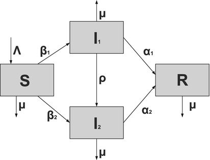
Mutation is accounted for in epidemic models through a term that transfers individuals infected with one of the strains into individuals infected with the other. To illustrate how mutation is treated in epidemic models, we introduce a two-strain SIR epidemic model with mutation. The model is very similar to the competitive exclusion model (8.1) but includes the mutation of strain-one-infected individuals into strain-two-infected individuals at a mutation rate ρ. The flowchart of the model is given in Fig. 8.3.

A304573_1_En_8_Fig3_HTML.gif


Fig. 8.3
Flowchart of a two-strain SIR epidemic model with mutation

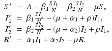
The model, first introduced in [25], is given below. The notation is the same as in model (8.1):


$$\displaystyle\begin{array}{rcl} S'& =& \varLambda -\beta _{1}\frac{SI_{1}} {N} -\beta _{2}\frac{SI_{2}} {N} -\mu S, \\ I_{1}'& =& \beta _{1}\frac{SI_{1}} {N} - (\mu +\alpha _{1}+\rho )I_{1}, \\ I_{2}'& =& \beta _{2}\frac{SI_{2}} {N} - (\mu +\alpha _{2})I_{2} +\rho I_{1}, \\ R'& =& \alpha _{1}I_{1} +\alpha _{2}I_{2} -\mu R. {}\end{array}$$

(8.12)

We mention that mutation incorporated in this way is modeled as a continuous event.


8.2.2 Superinfection


Superinfection is the process by which an individual that has previously been infected by one pathogen variant becomes infected with a different strain of the pathogen, or another pathogen at a later point in time. The second strain is assumed to “take over” the infected individual immediately. Thus this individual becomes infected with the second strain of the pathogen.

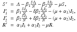
Superinfection is accounted for in epidemic models through a term that transfers individuals infected with one of the strains into individuals infected with the other. To illustrate how superinfection is treated in epidemic models, we introduce a two-strain SIR epidemic model with superinfection. The model is very similar to the competitive exclusion model (8.1) but includes the superinfection of individuals infected with strain one by individuals infected with strain two. The transmission rate β 2 at superinfection is reduced or enhanced by δ. If δ < 1, then the transmission rate β 2 is reduced; if δ > 1, then the transmission rate is enhanced. The flowchart of the model is given in Fig. 8.4.

A304573_1_En_8_Fig4_HTML.gif


Fig. 8.4
Flowchart of a two-strain SIR epidemic model with superinfection

The model, first introduced in [126], is given below. Notation is the same as in model (8.1):


$$\displaystyle\begin{array}{rcl} S'& =& \varLambda -\beta _{1}\frac{SI_{1}} {N} -\beta _{2}\frac{SI_{2}} {N} -\mu S, \\ I_{1}'& =& \beta _{1}\frac{SI_{1}} {N} -\delta \beta _{2}\frac{I_{1}I_{2}} {N} - (\mu +\alpha _{1})I_{1}, \\ I_{2}'& =& \beta _{2}\frac{SI_{2}} {N} +\delta \beta _{2}\frac{I_{1}I_{2}} {N} - (\mu +\alpha _{2})I_{2}, \\ R'& =& \alpha _{1}I_{1} +\alpha _{2}I_{2} -\mu R. {}\end{array}$$

(8.13)
In the above model, individuals infected with strain two can superinfect individuals infected with strain one. That is, individuals infected with strain one who come into contact with individuals infected with strain two can become immediately infected with strain two. One open question with the superinfection model (8.13) is what happens if the superinfection goes in both directions. To investigate this option, suppose in addition to strain two superinfecting strain one in the model above, we have that strain one also superinfects strain two. Hence model (8.13) takes the form


$$\displaystyle\begin{array}{rcl} S'& =& \varLambda -\beta _{1}\frac{SI_{1}} {N} -\beta _{2}\frac{SI_{2}} {N} -\mu S, \\ I_{1}'& =& \beta _{1}\frac{SI_{1}} {N} -\delta \beta _{2}\frac{I_{1}I_{2}} {N} +\delta _{1}\beta _{1}\frac{I_{1}I_{2}} {N} - (\mu +\alpha _{1})I_{1}, \\ I_{2}'& =& \beta _{2}\frac{SI_{2}} {N} +\delta \beta _{2}\frac{I_{1}I_{2}} {N} -\delta _{1}\beta _{1}\frac{I_{1}I_{2}} {N} - (\mu +\alpha _{2})I_{2}, \\ R'& =& \alpha _{1}I_{1} +\alpha _{2}I_{2} -\mu R. {}\end{array}$$

(8.14)
It can be seen that the two superinfection terms in each of the equations for I 1′ and I 2′ are the same except for their coefficients. This means that they can be combined. For instance,


$$\displaystyle{-\delta \beta _{2}\frac{I_{1}I_{2}} {N} +\delta _{1}\beta _{1}\frac{I_{1}I_{2}} {N} = \left (-\delta \beta _{2} +\delta _{1}\beta _{1}\right )\frac{I_{1}I_{2}} {N}.}$$
The constant coefficient is either positive or negative. If it is negative, it can be written as


$$\displaystyle{-\delta \beta _{2} +\delta _{1}\beta _{1} = -\hat{\delta }\beta _{2}.}$$
Hence, the equation for I 2′ takes the same form as in system (8.13). The expression in the equation for I 2′ in (8.14) is the same but with the opposite sign. We conclude that the symmetric system (8.14) is mathematically equivalent to the asymmetric system (8.13). For that reason, typically only the asymmetric system (8.13) is investigated.


8.2.3 Coinfection


Coinfection is the process of infection of a single host with two or more pathogen variants (strains) or with two or more distinct pathogen species. Coinfection with multiple pathogen strains is particularly common in HIV, but it occurs in many other diseases. Coinfection with multiple pathogen species is also thought to be a very common occurrence. Particularly widely distributed combinations are HIV and tuberculosis, HIV and hepatitis, HIV and malaria, and others. Coinfection is of significant importance because it may have negative effect both on the health of the coinfected individuals as well as on the public health in general. For instance, a coinfection of a human or a pig with human influenza strain and H5N1 strain may result in a pandemic strain, causing a widespread deadly pandemic.

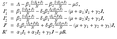
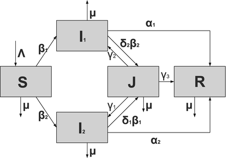
To model coinfection, we need to introduce a new dependent variable, namely J(t), the number of coinfected individuals in the population. The model again is built on the basis of the competitive exclusion model (8.1), but with a coinfected class J. Individuals infected with strain one can become coinfected with strain two and move to the coinfected class, and similarly for individuals originally infected with strain two. A typical assumption is that the probability of a susceptible individual getting infected with both strains simultaneously is too small and can be neglected. Both infected individuals with strain one and coinfected individuals can infect with strain one, and similarly with strain two. Recovery in a coinfection model is complex. Jointly infected individuals can recover from strain one, thereby moving to the class I 2, or they can recover from strain two and move to the class I 1. The possibility that jointly infected individuals recover from both classes also exists. In that case, they move to the recovered class R.

The flowchart of the model is given in Fig. 8.5. The model, previously introduced in [113], takes the form


$$\displaystyle\begin{array}{rcl} S'& =& \varLambda -\beta _{1}\frac{S(I_{1} + J)} {N} -\beta _{2}\frac{S(I_{2} + J)} {N} -\mu S, \\ I_{1}'& =& \beta _{1}\frac{S(I_{1} + J)} {N} -\delta _{2}\beta _{2}\frac{I_{1}(I_{2} + J)} {N} - (\mu +\alpha _{1})I_{1} +\gamma _{2}J, \\ I_{2}'& =& \beta _{2}\frac{S(I_{2} + J)} {N} -\delta _{1}\beta _{1}\frac{(I_{1} + J)I_{2}} {N} - (\mu +\alpha _{2})I_{2} +\gamma _{1}J, \\ J'& =& \delta _{1}\beta _{1}\frac{(I_{1} + J)I_{2}} {N} +\delta _{2}\beta _{2}\frac{I_{1}(I_{2} + J)} {N} - (\mu +\gamma _{1} +\gamma _{2} +\gamma _{3})J, \\ R'& =& \alpha _{1}I_{1} +\alpha _{2}I_{2} +\gamma _{3}J -\mu R. {}\end{array}$$

(8.15)


A304573_1_En_8_Fig5_HTML.gif


Fig. 8.5
Flowchart of a two-strain SIR coinfection model

Here some of the new parameters have the following meanings: δ i is a coefficient of reduction/enhancement of infection during coinfection, α i is the recovery rate of strain i during a single-strain infection, γ i is the recovery rate of strain i during coinfection, and γ 3 is the recovery of jointly infected individuals from both strains simultaneously.


8.2.4 Cross-Immunity


Cross-immunity is a form of immunity in which prior infection with one variant of the pathogen renders partial protection against another variant of the same pathogen or a different pathogen. Cross immunity, just like coinfection, can apply to strains of the same microorganism or can apply to different pathogen species. In the first case, the most notable example is influenza, where infection with one strain often provides some sort of immunity to other influenza strains. Mathematical models also have suggested that short-lived cross-immunity may exist among the four dengue serotypes [2]. In terms of cross-protective immunity between two distinct pathogens, mathematical models have suggested that such may exist between leprosy and tuberculosis [99]. Another example of cross-reactivity that has been confirmed in humans is one that involves the influenza virus and the hepatitis C virus [165].

To introduce the model, besides the traditional classes S, I 1, and I 2, there are also the classes of the recovered individuals from strain i, denoted by R i , the class J 2 of individuals recovered from strain one and now infected with strain two, and symmetrically, the class J 1 recovered from strain two and now infected with strain one, and finally, the class R of individuals recovered from both strains. The cross-immunity that strain i provides to strain j is incorporated in 
$$\sigma _{j}$$
.

Only gold members can continue reading. Log In or Register to continue

Stay updated, free articles. Join our Telegram channel

Nov 20, 2016 | Posted by in PUBLIC HEALTH AND EPIDEMIOLOGY | Comments Off on Multistrain Disease Dynamics

Full access? Get Clinical Tree

Get Clinical Tree app for offline access