- Fluctuation The profile appears as a series of peaks and troughs, known as fluctuation. The peaks occur at the time a dose is given, and the troughs occur immediately before the next dose.
- Accumulation It can be seen in Figure 12.1 that the troughs and peaks increase with each dose, known as accumulation. This occurs when a dose is given at a time when drug from a previous dose is still in the body. Note that there is less accumulation with each successive dose.
- Steady state Eventually, accumulation between doses stops altogether. At this time, the peaks and troughs with successive doses are the same; that is, steady state has been achieved.
- Average Cp Note that the average plasma concentration throughout therapy (indicated by the dashed line in Figure 12.1) has the same shape as the plasma concentration–time profile of a continuous constant infusion.
The goal of drug therapy is to devise a dosing regimen that will maintain therapeutic steady-state plasma concentrations. A multiple-dosing regimen consists of two parts: (1) the dose and (2) the dosing interval, or the frequency with which the doses are repeated. For example, in Chapter 11 it was found that a constant continuous infusion of 3.1 mg/h of the fictitious drug lipoamide would provide a therapeutic plasma concentration of 50 μg/L (see Problem 11.5). It has been found that plasma concentrations of lipoamide greater than 90 μg/L are associated with a high frequency of side effects. Plasma concentrations below 25 μg/L are subtherapeutic. If multiple discrete doses of lipoamide are to be given, what dose and what dosing interval should be used to ensure that plasma concentrations are therapeutic and nontoxic at all times? The material presented in this chapter is directed at answering this question.
12.2 TERMS AND SYMBOLS USED IN MULTIPLE-DOSING EQUATIONS
The formulas for multiple-dosing pharmacokinetics introduce some new symbols. These are shown in Figure 12.2 and described below.
FIGURE 12.2 Symbols used in multiple-dose pharmacokinetics. In this example, the dose is administered every 8 h. n is the number of the last dose administered, τ the dosing interval (8 h), and t the time since the last dose (in this regimen, t will vary continuously from 0 through 8 h). Cpmin,n and Cpmin,ss the trough plasma concentrations (t = τ) before and after steady state, respectively; Cpmax,n and Cpmax,ss are the peak plasma concentrations (t = 0) before and after steady state, respectively.
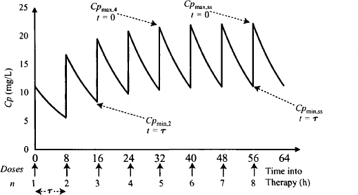
- n is the number of the last dose administered.
- τ (the lowercase Greek letter tau) is the dosing interval. If 50 mg is administered every 8h, τ is 8 h.
- t is the time since the last dose. During therapy, t varies continuously from 0 at the beginning of a dosing interval to τ at the end. When the next dose is given, t once more becomes 0.
- Time into therapy can be calculated from the product of n · τ. Specifically, time into therapy = [(n – 1) · τ] + t. For example let τ = 12; then:
- Peak plasma concentrations, which occur when t = 0, have the symbol Cpmax. Before steady state, Cpmax is dependent on the number of the last dose, so it has the symbol Cpmax,n. After steady state, the peak is independent of the number of the last dose and has the symbol Cpmax,ss.
- Trough plasma concentrations, which occur when t = τ, have the symbol Cpmin. Before steady state, Cpmin is dependent on the number of the last dose and has the symbol, Cpmin,n. After steady state, the peak is independent of the number of the last dose and has the symbol Cpmin,ss.
- The symbols, Cpn and Cpss are used to represent the plasma concentration at any other time during a non-steady-state and a steady-state dosing interval, respectively.
The derivation of the equations for multiple doses involves a number of assumptions, which include:
Thus, these equations can only be applied to situations where the assumptions hold. For example, the equations should not be used for drugs that display nonlinear pharmacokinetics, such as phenytoin (Chapter 15).
12.3 MONOEXPONENTIAL DECAY DURING A DOSING INTERVAL
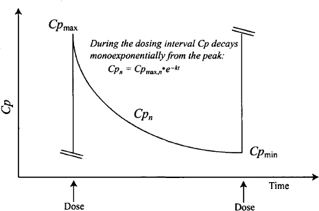
When a dose is administered, it is assumed that the entire dose enters the systemic circulation at time zero, even though in reality an injection may be given gradually over a period of a minute or more. For the one-compartment model, the drug is assumed to distribute in a rapid, essentially instantaneous manner. Thus, the: peak plasma concentration is assumed to occur at time zero. During a dosing interval, t increases from zero at the time of the dose up to its maximum value of τ just before the next dose. During this period, the plasma concentration is under the influence of only one process: first-order elimination (Figure 12.3). During a dosing interval, the plasma concentration decays monoexponentially from the peak (Cpmax) to the trough (Cpmin).
FIGURE 12.3 Monoexponential decay during a dosing interval. During a dosing interval, plasma concentrations are influenced only by first-order elimination. As a result, they decay monoexponentially from the peak. The first-order decay equation can be used to express the plasma concentration during the interval as a function of the peak concentration and the time after the dose.
Before steady state, during a dosing interval,
(12.1) 
and at the trough,
(12.2) 
At steady state, during a dosing interval,
(12.3) 
and at the trough,
This basic relationship between the plasma concentration and time during a dosing interval permits the simple derivation of an important equation that is used to calculate dosing intervals needed to achieve certain peak and trough plasma concentrations.
12.3.1 Calculation of Dosing Interval to Give Specific Steady-State Peaks and Troughs
Knowing that the fall in the plasma concentration between doses is simple monoexponential decay makes it possible to calculate the value of a dosing interval to give specific peaks and troughs. This is best addressed through an example.
Example 12.1 Assume that a new drug is under development. It has a very narrow therapeutic range (12 to 25 mg/L). However, since it is being used to treat a serious life-threatening condition for which few other treatments are available, development of this drug is being pursued. The goal is to design a dosing regimen that will result in a steady-state peak and trough of 20 and 14 mg/L, respectively. The drug’s elimination rate constant has a population average value of 0.043 h−1. What dosing interval is needed to provide the desired steady-state peaks and troughs?
Solution The relationship between the steady-state peak and trough is given in equation (12.4). Substituting the desired steady-state trough and peak into this equation gives us
A more useful arrangement of equation (12.4) for use in calculating a dosing interval is
The box around equation (12.5) indicates that it is an important equation that is in frequent use clinically.
12.4 BASIC PHARMACOKINETIC EQUATIONS FOR MULTIPLE DOSES
12.4.1 Principle of Superposition
When a dose of a drug is administered at a time when drug from a previous dose(s) is still in the body, it is assumed that the total amount of drug in the body is equal to the amount provided by the new dose, plus the drug remaining from previous dose(s). This is known as the principle of superposition, illustrated in Table 12.1 for a drug that is administered as a 64-mg dose every half-life. At the end of the first dosing interval, half (32 mg) of the first dose remains. So the peak amount after the second dose is the dose (64 mg) plus that remaining from the first dose (32 mg), or 96 mg. The same process can be used to calculate the next trough amount and the peaks and troughs after successive doses as shown in Table 12.1. Note that after the first dose the body accumulates 32 mg, but there is less accumulation with each dose. For example, in Table 12.1 it can be seen that only 2 mg is accumulated between the fifth and sixth doses. Eventually, no further accumulation occurs, and steady state is achieved. At steady state an entire dose (64 mg) is lost during a dosing interval, only to be replaced exactly by the next dose.
TABLE 12.1 Maximum (Abmax) and Minimum (Abmin) Amounts of Drug in the Body and Accumulation After Successive Doses of 64 mg Are Given Every Half-Life
12.4.2 Equations That Apply Before Steady State
The equations for multiple intravenous bolus injections are derived using exactly the same process as that described above; the full derivation appears in Appendix D. The basic equation that can be used to determine the plasma concentration at any time during multiple-dose therapy is
Recall that t is the time that has elapsed since the last dose, n the number of the last dose, and τ the dosing interval. When t = 0, a peak plasma concentration is observed:
When t = τ, a trough is observed:
Alternatively, the trough may be expressed as
Example 12.2 Multiple intravenous bolus injections (250 mg) of a drug are administered every 8 h. The drug has the following parameters: S = 1, Vd = 30 L, k = 0.1 h−1, and τ = 8 h. Calculate:
Solution
12.5 STEADY STATE
Usually, steady state is the focus of drug therapy and the goal is to achieve steady-state plasma concentrations that are in the therapeutic range. Consequently, the equations associated with steady state are very important and are more commonly used clinically than the equations that apply prior to steady state. The specific aspects of steady state that are of most interest are the determinants of:
- The steady-state peak and trough plasma concentrations
- The average plasma concentration during a steady-state dosing interval
- The factors that control the amount of fluctuation observed at steady state (Cpmax,ss versus Cpmin,ss)
- The degree of accumulation that ultimately occurs at steady state
- The time to reach steady state
12.5.1 Steady-State Equations
At steady state, the plasma concentration–time profile is exactly the same for all dosing intervals (i.e., the plasma concentrations become independent of n, the number of the last dose). Recall the basic equation that applies before steady state:
(12.10) 
During therapy n increases with each successive dose. As a result, as therapy progresses and steady state is approached, e−nkτ tends to zero, and 1 – e−nkτ becomes 1 and disappears from the equation. Thus, the basic equation for steady state is expressed
(12.11) 
The corresponding equation for the peak and trough may be expressed by letting t = 0 and τ, respectively:
or
Example 12.3 Next continuing with our example of a drug (Vd = 30 L, k = 0.1 h−1) that is administered intravenously as 250 mg administered every 8 h. Recall that after the second dose,
Calculate the maximum and minimum steady-state plasma concentrations achieved by the regimen.
Solution
The steady-state peaks and troughs are 15.1 and 8.8 mg/L, respectively.
These equations can also be used in the reverse direction to determine a dose to produce a desired steady-state peak and/or trough.
Example 12.4 Recall that it was determined earlier (Example 12.1) that a dosing interval of 8.3 h (approximately 8 h) was needed for a drug (Vd = 50 L, k = 0.043 hr−1) to achieve steady-state troughs and peaks of 14 and 20 mg/L, respectively. What dose should be used?
Solution Either the formula for Cpmax,ss or that for Cpmin,ss can be used. The only unknown in either case is the dose:
or

Assuming that S = 1, F = 1,
The intravenous injection of 290 mg of this drug every 8 h should result in a steady-state peak and trough of 20 and 14 mg/L, respectively.
12.5.2 Average Plasma Concentration at Steady State
Frequently, rather than concentrating on the peaks and troughs, the emphasis of multiple dosing therapy is to achieve a desired therapeutic average steady-state plasma concentration. For example, digoxin has a very long half-life, and plasma concentrations remain fairly consistent during a dosing interval. It is often necessary to determine the dose needed to achieve an average plasma concentration of 1 μg/L. It would be useful to have an expression that relates the average steady-state plasma concentration to the dose and dosing interval.
Because the fall in Cp
Stay updated, free articles. Join our Telegram channel

Full access? Get Clinical Tree


