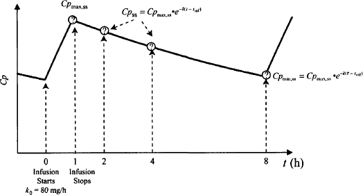
FIGURE 13.2 Multiple intermittent infusions: plasma concentrations during a steady-state dosing interval. Time t is the time after the start of the infusion. The dosing interval can be separated into two periods: A and B. During period A the infusion is running and plasma concentrations increase. Note that the peak occurs when the infusion stops (t = t_inf). During period B (from t = t_inf to t = τ), there is no ongoing drug input, and plasma concentrations decay monoexponentially.

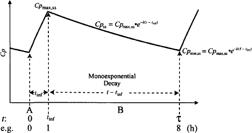
The symbols used are the same as those used for bolus injections: t is the time that has elapsed since the dose was administered (start of the infusion) and τ is the dosing interval or time between doses. Tau varies constantly from zero to τ, to zero to τ, and so on. The equations for multiple infusions incorporate an additional time parameter, the duration of the infusion (t_inf). The dosing interval can be broken down into two parts: the period from time 0 to t_int when the infusion is running, during which plasma concentrations increase (A in Figure 13.2); and the period from the end of the infusion to the end of the dosing interval (period t_inf to τ) when the infusion is not running. During the latter period, plasma concentrations fall monoexponentially under the influence of first-order elimination (B in Figure 13.2). Note in Figure 13.2 that the peak occurs when t = t_inf, and a trough is obtained at the end of the dosing interval when t = τ.

In a dosing interval, once the infusion stops, the plasma concentration falls monoexponentially from the peak. As a result, the plasma concentration at any time during this period (B in Figure 13.2) can be expressed in terms of its decay from the peak and the time that has elapsed from the peak (t – t_inf). For example, at steady state:

(13.1)

where Cp_ss is the concentration at any time, t, during the dosing interval and Cp_max,ss is the steady-state peak. Cp at the trough during a steady-state dosing interval (Cp_min,ss) is expressed as

(13.2)

13.2 STEADY-STATE EQUATIONS FOR MULTIPLE INTERMITTENT INFUSIONS

In Chapter 12 we demonstrated that an equation for multiple dosing could be constructed as follows (Figure 12.6):

Expressions for the fraction of steady state achieved at any time and the final accumulation at steady state were derived in Chapter 12 [equations (12.27) and (12.23), respectively]. Thus,

(13.3)

If the equation is to be limited to steady state, the fraction of steady state (1 – e^−nkτ) equals 1 and can be removed from the expression:

(13.4)

The equation for the plasma concentration at any time after a single infusion was presented in Chapter 11 [equation (11.16)]:

(13.5)

where T is the time the infusion was terminated and t’ is the time elapsed since termination. Next we substitute the time symbols used for multiple infusions: T = t_inf and t’ = t – t_inf. Substituting these symbols into equation (13.5) and then substituting into equation (13.4) yields

(13.6)

where Cp_ss is the plasma concentration at any time during a steady-state dosing interval, k₀ the infusion rate, S the salt factor of the drug, F the bioavailability, k the elimination rate constant, t_inf the duration of the infusion, t the time elapsed since the infusion was started, Cl the clearance, and τ the dosing interval or time between the start of consecutive infusions.

A peak plasma concentration occurs at the end of the infusion when t = t_inf:

(13.7)

A trough plasma concentration occurs at the end of the dosing interval (t = τ), immediately before the next infusion is started:

(13.8)

Example 13.1 A drug (Cl = 8.67 L/h; Vd = 100 L; and S = 1) was administered as multiple intravenous infusions. The dose (80 mg) was administered over a 1-h period every 8 h. Calculate the estimated plasma concentrations in the third day of therapy, at (a) 1 h, (b) 2 h, (c) 4 h, and (d) 8 h after the start of the first infusion of the day.

Solution The drug has a t_1/2 = 0.693 × 100/8.67 = 8 h. A dose of 80 mg is infused over 1 h: k₀ = 80 mg/h. S = 1, F = 1. The problem is summarized in Figure 13.3. It will take about 24 to 40 h to get to steady state. By the third day, steady state will have been achieved and the profiles from the three infusions of the day will be exactly the same.

FIGURE 13.3 Example problem using multiple intermittent infusion equations. The drug is administered at a rate of 80 mg/h over a 1-h period. Plasma concentrations at 1,2, 4, and 8 h must be calculated after the first dose on the third day.

Example 13.2 A 0.5 h infusion is used to administer the dose (80 mg) of the drug described in Example 13.1. Calculate the estimated plasma concentrations on the third day of therapy, at (a) 0.5 h, (b) 1 h, (c) 2 h, and (d) 8 h after the start of the infusion.

Solution The drug has a t_1/2 = 0.693 × 100/8.67 = 8 h. A dose of 80 mg is infused over 0.5 h: k₀ = 160 mg/h. S = 1, F = 1. It will take about 24 to 40 h to get to steady state. By the third day, steady state will have been achieved. A diagram of the steady-state dosing interval is shown in Figure 13.3 but in this example t_inf = 0.5 h.

(a) When t = 0.5, the infusion has just been terminated, Cp = Cp_max,ss

Only gold members can continue reading. Log In or Register to continue

Share this:

• Click to share on Twitter (Opens in new window)
• Click to share on Facebook (Opens in new window)

Like this:

Like Loading...

Related

Related posts:

1. Drug Administration, Absorption, and Bioavailability
2. Introduction to Pharmacodynamic Models and Integrated Pharmacokinetic–Pharmacodynamic Models
3. Drug Distribution
4. Drug Elimination and Clearance

Stay updated, free articles. Join our Telegram channel

Join