Multiple-Dose Regimens

OBJECTIVES

The reader will be able to:

• Define the meaning of the following words and phrases: drug accumulation, accumulation index, acquired resistance, average level at plateau, loading dose, maintenance dose, multiple-dose regimen, priming dose, relative fluctuation, trough concentration.
  
• Predict the plasma concentration–time profile following a fixed-dose and fixed–dosing-interval regimen when given the plasma concentration–time profile after a single dose of drug.
  
• Design a dosage regimen from knowledge of the pharmacokinetics and therapeutic window of a drug.
  
• Predict the rate and extent of drug accumulation for a given regimen of fixed dose and fixed interval.
  
• Explain why the time to reach plateau on a multiple-dosing regimen depends only on the half-life of the drug.
  
• Discuss the rationale behind a loading dose, and calculate the maintenance dose needed to maintain therapeutic levels knowing the half-life and the loading dose of the drug, and vice versa.
  
• Offer three examples of drugs for which the dosage regimen is conditioned by the half-life of the drug and its therapeutic index.
  
• Discuss the application of modified-release products to the development of more convenient dosage regimens.
  
• Explain why the time to reach a plateau of effect following a multiple-dose regimen is sometimes governed more by the pharmacodynamics than the pharmacokinetics of a drug, and give two examples illustrating this situation.
  
• Discuss how tolerance to the desired or adverse effects of a drug impacts on the optimal design and use of multiple-dose regimens.
  
• Give an example of a situation that requires intermittent drug administration for optimal therapy.

he previous chapter dealt with constant-rate regimens. Although these regimens possess many desirable features, they are not the most common ones. The more common approach to the attainment and maintenance of continuous or chronic therapy is to give multiple discrete doses. This chapter covers the pharmacokinetic principles associated with such multiple dosing and, together with pharmacodynamics, the establishment of appropriate multiple-dose regimens. Also covered is the design and application of regimens using modified-release dosage forms.

PRINCIPLES OF DRUG ACCUMULATION

Drugs are most commonly prescribed to be taken on a fixed-dose, fixed–time-interval basis, for example, 50 mg 3 times a day, or 20 mg once a day. Associated with this kind of administration, the plasma concentration and amount in the body fluctuate and, similar to an infusion, rise toward a plateau.

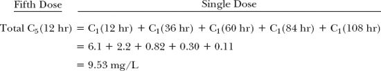
To appreciate what happens when such regimens are taken, consider the plasma concentration–time data over 120 hr (5 days) in Table 11-1, also displayed in Fig. 11-1, following the oral administration of a single 200-mg dose of a drug. This drug is relatively slowly eliminated, is completely absorbed, and because it is very rapidly absorbed, the peak concentration occurs at the first time of measurement, 1 hr after administration. The intention is to give the same dose of this drug once daily. We wish to predict the anticipated concentrations over the first 5 days. To do this, we expect the concentration–time profile associated with each dose to be the same as that following the first dose, except that each profile will be displaced in time by the number of days since the first dose was given, as listed in Table. 11-1 and shown as dotted lines in Fig. 11-1. The observed plasma concentration–time profile is then the sum of the concentrations associated with each of the doses. These are listed in the last column of Table. 11-1. For example, the concentration at 1 hr after the second dose (25 hr since the first dose) is the sum of that remaining from the first dose at 25 hr (3.5 mg/L) plus that associated with the second dose at 1 hr after dosing (9.6 mg/L), or 13.1 mg/L. Similarly, the concentration at 12 hr after the fifth dose, or 108 hr (4 × 24 + 12) after the first dose, is given by where the subscript denotes the dose number, and the value in parenthesis denotes the time since that dose was administered.

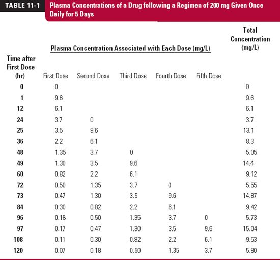
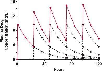
FIGURE 11-1. Accumulation on approach to plateau. When the plasma concentration–time profile is known following a single dose of drug, the anticipated profile following repetitive administration of a fixed dose of drug given at regular intervals can be calculated by replicating the single dose profile after each new dose (black dashed lines) and summing at each time the resultant concentrations associated with each dose. The result (colored lines) is a typical sawtooth profile rising to a plateau. The data used to generate these profiles are given in Table. 11-1.

Several points are worth noting. First, clear evidence of accumulation in the plasma concentration is seen resulting in a characteristic rising sawtooth profile, showing fluctuation in concentration within each dosing interval. This accumulation occurs because there is always some drug left in the body from previous doses. Second, accumulation continues until a plateau is reached, after which time there is no further increase in the concentration from one dosing interval to the next. Analysis of the data in Table. 11-1 shows that this occurs because by that time, about 4 days in the current example, virtually nothing is left in the body from the first dose. This pattern thus repeats itself for each subsequent dosing interval. Lastly, this calculation requires no knowledge of any pharmacokinetic parameter, be it clearance, volume of distribution, or oral bioavailability. All that is needed is the profile after a single dose, irrespective of its shape or complexity. This is the main attraction of this approach. Its limitation is that the calculations are restricted to the same times after each dose as that observed following the single dose. We now consider a direct method of calculating the amount of drug in the body and the plasma concentration at any time after any number of doses, starting with repetitive administration of intravenous (i.v.) bolus doses.

MAXIMA AND MINIMA ON ACCUMULATION TO THE PLATEAU

To appreciate further the phenomenon of accumulation, consider what happens when a 100-mg bolus dose is given intravenously (see Chapter 3, Kinetics After an Intravenous Bolus Dose) every elimination half-life. To simplify matters, we again start with administration into the well-stirred reservoir model considered in Chapter 5, Elimination. The events are depicted in Fig. 11-2. The amounts in the body just after each dose and just before the next dose can readily be calculated; these values correspond to the maximum (A_max) and minimum (A_min) amounts obtained within each dosing interval. The corresponding values (black line) during the first dosing interval are 100 mg (A_max,1) and 50 mg (A_min,1), respectively. The maximum amount of drug in the second dosing interval (A_max,2), 150 mg, is the dose (100 mg) plus the amount remaining from the previous dose (50 mg). The amount remaining at the end of the second dosing interval (A_min,2), 75 mg, is that remaining from the first dose, 25 mg (100 mg × ½ × ½, because two half-lives have elapsed since its administration) plus that remaining from the second dose, 50 mg. Alternatively, the value, 75 mg, may simply be calculated by recognizing that one-half of the amount just after the second dose, 150 mg, remains at the end of that dosing interval. Upon repeating this procedure, it is readily seen (curve B, Fig. 11-2) that drug accumulation, viewed in terms of either maximum or minimum amount in the body, continues until a limit is reached. At the limit, the amount lost in each interval equals the amount gained, the dose. In this example, the maximum and the minimum amounts in the body at steady state are 200 and 100 mg, respectively. This must be so because the difference between the maximum and minimum amounts is the dose, 100 mg, and because at the end of the interval, one half-life, the amount must be one half that at the beginning.

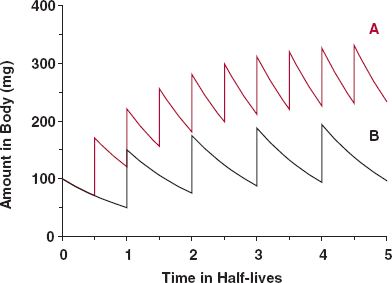
FIGURE 11-2. Dosing frequency controls the degree of drug accumulation. Intravenous bolus dose (100 mg) administered once every half of a half-life (A, colored line); same bolus dose administered once every half-life (B, black line). Note that time is expressed in half-life units.

Recall, following a constant-rate input, that the plateau is reached when rate of elimination matches rate of input. Then, the level of drug in the body is constant as long as the input rate is maintained. With discrete dosing, the level is not constant within a dosing interval, but the values at a given time within the interval are the same from one dosing interval to another. The term plateau is also applied to this interdosing steady-state condition.

The foregoing considerations can be expanded for the more general situation in which a drug is given at a dosing interval, τ, not equal to the half-life. The general equations are derived in Appendix I, Amount of Drug in Body on Accumulation to Plateau, for the maximum and minimum amounts in the body after the Nth dose (A_max,N; A_min, _N) and at steady state (A_max,ss; A_min,ss). These are

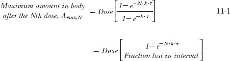
Recall from Chapter 3, Kinetics Following an Intravenous Bolus Dose, that the function e^−kτ is the fraction of the initial amount remaining in the body at time t. So that 1– e^−k·τ is the fraction of drug lost during a dosing interval τ. Similarly, the amount in the body at the end of a dosing interval τ of a multiple-dose regimen, (A_{min N}), frequently called the trough value, is obtained by multiplying the corresponding maximum amount by e^–k·τ, that is, A_{min, N} = A_max,N · e^−Kτ or A_min,ss = A_max,ss · e_−Kτ.

The corresponding values for the plasma concentration are obtained by dividing the equations above by the volume of distribution of the drug. Returning to the example in Table. 11-1, which approximates an i.v. bolus situation, the half-life of this drug, gained from a semilogarithmic plot of the plasma concentration after the single dose, is 16.7 hr and its volume of distribution is 20 L. Given this information, it is readily seen that the maximum and minimum concentrations anticipated at plateau, C_max,ss and C_min,ss, when the 200-mg dose is given once daily (every 24 hr) are, by substitution

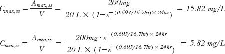
Notice that the previously calculated maximum and minimum values after the fifth dose (15.1 and 5.8 mg/L; Table. 11-1) are very close to the correspondingly predicted maximum and minimum plateau concentrations, indicating that for all practical purposes (≥90%, as with constant-rate input) a plateau is anticipated to be reached by day 5 of dosing for this drug. Also, it is apparent that Eq. 11-3, upon dividing by V, offers a rapid way of calculating the maximum exposure likely to occur with a given dosage regimen, once the pharmacokinetic parameters of a drug following a single dose are known.

Equations 11-1 to 11-4 strictly apply only to intravascular bolus administration. They are reasonable approximations following extravascular administration when, as in the above example, absorption is complete and rapid relative to elimination. The following discussion deals with a less restrictive view of accumulation, which applies to all routes of administration.

AVERAGE LEVEL AT PLATEAU

In many respects, the accumulation of drugs administered in multiple doses is the same as that observed following constant-rate input. The average amount in the body at plateau is readily calculated using the steady-state concept: average rate in must equal average rate out. The average rate in is F · Dose/τ, where Fis the bioavailability of the drug. The average rate out is k · A_av,ss, where A_av,ss is the average amount of drug in the body over the dosing interval, τ, at plateau. Therefore,

or

where C_av,ss is the average plasma concentration at plateau. Because k = 0.693/t_1/2, it also follows that

while rearranging Eq. 11-6 yields

These are fundamental relationships; they show how the average amount in the body at steady state depends on rate of administration (Dose/τ), bioavailability, and half-life, and how the corresponding average concentration depends on the first two factors and clearance. Returning to the first example, with a half-life of 16.7 hr (= 0.7 days), τ = 1 day, the average amount in the body at plateau is 200 mg. This amount lies approximately midway between the maximum and minimum amounts of 316 and 116 mg (calculated by multiplying the respective concentrations by the volume of distribution, 20 L). Notice also that, as expected, the difference between the maximum and minimum amounts is the dose, in this case, 200 mg. That A_av,ss = Dose in this example is fortuitous. Had, for example, F = 0.5 or the dosing interval been changed from 1 day to 12 hr, thereby doubling the frequency of administration, then clearly the equality between A_av,ss and Dose would disappear.

Drug accumulation is not a phenomenon that implicitly depends on the property of a drug, nor are there drugs that are cumulative and others that are not. Accumulation, particularly the extent of it, is a result of the frequency of administration relative to half-life (t1/₂/τ or 1/kτ) as shown in Fig. 11-2. Here, we see that by halving the dosing interval from one half-life to one half of a half-life (curve A), the extent of accumulation has doubled. Notice, however, that the time to reach the plateau has not changed.

For convenience and to assure adherence to a regimen, drugs are commonly given once or twice a day, with 3 and 4 times daily being less desirable. As a consequence, extensive drug accumulation is more common for those drugs with half-lives greater than 1 day. It is particularly noticeable when the half-life of the drug is much longer than 1 day.

RATE OF ACCUMULATION TO PLATEAU

The amount in the body rises on multiple dosing just as it does following constant-rate input (Chapter 10, Constant-Rate Input). That is, the approach to the plateau depends solely on the drug’s half-life. The simulation for the antiepileptic drug phenobarbital, in Table. 11-2, which shows the ratio of the minimum amount during various dosing intervals to the minimum amount at plateau, illustrates this point. This drug has a half-life of 4 days and is given at a dose of 100 mg once daily. Observe that it takes one half-life (4 days), or 4 doses, to be at 50% of the value at plateau, two half-lives (8 days), or 8 doses, to be at 75% of the plateau value, and so on.

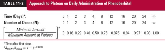
Accumulation of phenobarbital takes a long time because of its long half-life. Although once a day appears to be infrequent, relative to regimens of some drugs, it is frequent relative to phenobarbital’s half-life of 4 days. The degree of accumulation is extensive because of relatively frequent administration. The frequent administration also determines the small relative fluctuation in the amount of drug in the body at plateau, seen as the difference between the maximum and minimum values relative to the average. At plateau, 100 mg of phenobarbital is lost every dosing interval, the dose, which is small compared with the maximum and minimum amounts (from Eqs. 11-3 and 11-4) in the body at plateau, namely 630 and 530 mg.

The approach to steady state, observed for the minimum amounts of phenobarbital in the body, also holds true for the maximum amounts (proof in Appendix I, Amount of Drug in Body on Accumulation to Plateau) that is, on dividing Eq. 11-1 by Eq. 11-3, and Eq. 11-2 by Eq. 11-4:

By recognizing that N·τ is the total time elapsed since starting administration, expressed in multiples of the dosing interval, the similarity of Eq. 11-9 to the equation describing the rise of drug in the body to plateau following a constant-rate infusion (1 – e^−k·t; Eq. 10-9) becomes apparent. This point is further illustrated by the events depicted in Fig. 11-3. Here, the average dosing rate is maintained at 100 mg a day, but the drug is given with increasing frequency, which, in the limiting case of the dosing interval becoming infinitesimally small, is a constant-rate input. It is seen that the time course of average amount in the body is the same in all cases, but the less frequent the administration, the greater is the fluctuation.

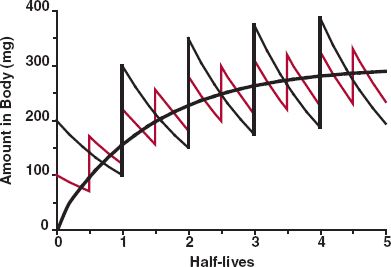
FIGURE 11-3. Plot showing that the time course of approach of amount in the body to the plateau is independent of the dosing interval. Here, the same average dosing rate was administered with increasing frequency, such that ultimately the dosing interval is so short as to approach that of a constant-rate input (smooth black line). Although the degree of fluctuation around the average value within a dosing interval varies with the dosing interval, the time to reach the plateau does not.

ACCUMULATION INDEX

When the amounts at steady state are compared with the corresponding values after the first dose, a measure of the extent of accumulation is obtained. This value can be thought of as an accumulation index (R_ac),

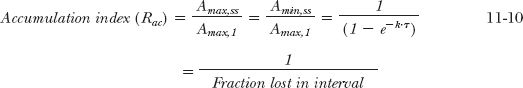
Thus, the quantity, 1/(1 – e^−kτ), is the accumulation index. When phenobarbital is given once daily (k = 0.173 day₋₁, τ = 1 day), the accumulation index is 5.8. Thus, the maximum and minimum amounts (and, for that matter, the amount at any time within the dosing interval at plateau) are 5.8 times the values at the corresponding times after a single dose.

CHANGE IN REGIMEN

Sometimes the dose of drug has to be changed, because the response is inadequate or excessive. Suppose, for example, that the decision is made to double the amount of phenobarbital in the body at plateau. The need for a twofold increase in the rate of administration, from 100 to 200 mg/day, follows from Eq. 11-7. However, due consideration has to be given to the time needed to achieve a new plateau on changing the dosing rate. This often guides how long one needs to wait to ensure the achievement of the full response associated with the change, before deciding if any further adjustments in drug therapy are needed. As with i.v. infusion, it takes one half-life to go one-half the way from the original plateau to the new one, two half-lives to go three quarters of the way, and 3.3 half-lives to reach plateau practically. For phenobarbital, it would take about 14 days (3.3 half-lives) to go from the original plateau (A_max,ss = 630 mg; A_min,ss = 530 mg) to greater than 90% of the way toward the new one (A_max,ss = 1260 mg; A_min,ss = 1060 mg) on doubling the daily dose. Hence, we would not expect to see the full benefits associated with this increase in dose for at least 2 weeks.

RELATIONSHIP BETWEEN INITIAL AND MAINTENANCE DOSES

It is sometimes therapeutically desirable to establish the required amount of drug in the body as soon as possible, rather than wait for this to be achieved by repeatedly giving the same dose at a regular interval. When a larger first or initial dose is given to quickly achieve a therapeutic level, it is referred to as priming or loading dose. A case in point is sirolimus (Rapamune), an immunosuppressive drug used as part of therapy to prevent rejection following organ transplantation. Sirolimus has a half-life on the order of 2.5 days, and the usual oral maintenance dose is 2 mg once a day. Given in this manner, it would take approximately 1 week to reach the plateau, which is much too long to prevent the increased risk of organ rejection. Instead, patients first receive a loading dose of 6 mg followed by 2 mg daily. Another example is digoxin used in the treatment of chronic atrial fibrillation; it has a half-life on the order of 2 days, and the usual oral maintenance dose is 0.25 mg taken once a day. Taken in this manner, it would take approximately a week to reach the plateau. In some patients, it is important to reach effective levels in the body relatively rapidly. In this case, digoxin is given as a larger initial dose, followed by the regular daily doses. For digoxin, the initial oral dose, up to 1 mg, is often administered in divided doses. Several procedures are followed, but the divided dose is commonly given every 6 hr until the desired therapeutic response is obtained. In this way, each patient is titrated to his or her required initial therapeutic dose.

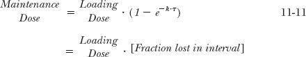
Instead of determining the loading dose when the maintenance dose is given, it is more common to determine the maintenance dose required to sustain a therapeutic amount in the body. The initial dose rapidly achieves the therapeutic response; subsequent doses maintain the response by replacing drug lost during the dosing interval. The maintenance dose, D_M, therefore, is the difference between the loading dose and the amount remaining at the end of the dosing interval, D_L · e^−kτ, that is,

Likewise, if the maintenance dose is known, the initial dose can be estimated:

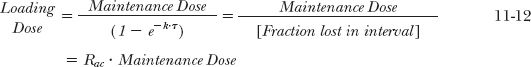
The relationship between loading dose and accumulation index, R_ac, follows from Eq. 11-10. For sirolimus, Eq. 11-12 predicts that a daily maintenance dose of 2 mg requires a loading dose of 8 mg. As noted previously, clinical experience indicates that a slightly lower dose (6 mg) suffices.

The similarity between Eqs. 11-3 and 11-12 should be noted. From the viewpoint of accumulation, Eq. 11-3 relates to the maximum amount at plateau on administering a given dose repetitively. If the maximum amount were put into the body initially, then Eq. 11-11 indicates the dose needed to maintain that amount. The relationships are the same, although they were derived starting from different viewpoints. These equations form the heart of multiple-dose administration.

The ratio of loading to maintenance doses depends on the dosing interval and the half-life and is equal to the accumulation index, R_ac (Eq. 11-12). For example, the antibiotic doxycycline has approximately a 1-day half-life, and a dose in the range of 200 mg is considered to provide effective antimicrobial drug concentrations. Therefore, a reasonable schedule is 200 mg (two 100-mg capsules) initially, followed by 100 mg once a day, as shown in Fig. 11-4. (In practice, it is recommended that the initial dose be divided into 100 mg taken 12 hr apart.) A dosage regimen, such as that for doxycycline, consisting of a priming dose equal to twice the maintenance dose and a dosing interval of one half-life, is convenient for drugs with half-lives between 8 and 24 hr. The frequency of administration for such drugs varies from 3 times a day to once daily, respectively. For drugs with half-lives less than 3 hr, or with half-lives greater than 24 hr, this regimen is often impractical.

Although a loading or initial dose greater than the maintenance dose seems appropriate for drugs with half-lives longer than 24 hr, such is often not the case. There are various reasons why this is so, which are discussed at greater length later in this chapter and also in Chapter 18, Initiating and Maintaining Therapy. Here, we note a few examples. For piroxicam, an analgesic/antipyretic drug with a half-life of 2 days, the most common adverse effects are gastrointestinal reactions. Such reactions may be increased if a loading dose, which would be 3 to 4 times the maintenance dose (Eq. 11-12, τ= 1 day), is given. Another example is that of protriptyline (an antidepressant with a half-life of 3 days), for which larger doses slow gastric emptying and gastrointestinal activity (anticholinergic effect), resulting in slower and more erratic absorption of this and other drugs.

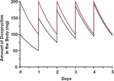
FIGURE 11-4. Sketch of the amount of doxycycline in the body with time in an individual with a 24-hr half-life following i.v. administration of 200 mg initially and 100 mg once daily thereafter (colored line). When the initial and maintenance doses are the same, it takes 4 days (four half-lives) before the plateau is practically reached (black line). Thereafter, the two curves are essentially the same.

MAINTENANCE OF DRUG IN THE THERAPEUTIC RANGE

Dosage regimens that achieve effective therapy for drugs with both high and medium-to-low therapeutic indices and with various half-lives are listed in Table. 11-3.

HALF-LIVES LESS THAN 30 MINUTES

Great difficulty is encountered in trying to maintain therapeutic levels of such drugs. This is particularly true for a drug with a low therapeutic index, for example, heparin and esmolol, which have half-lives of approximately 30 and 10 min, respectively. Such type of drugs must be either infused or discarded unless intermittent systemic exposures are permissible. Drugs with a high therapeutic index may be given less frequently, but the longer the dosing interval, the greater is the maintenance dose required to ensure that drug in the body stays above a minimum effective value, and the greater is the degree of fluctuation. Penicillin is a notable example of a drug for which the dosing interval (4–6 hr) is many times longer than its half-life (~30 min). This is possible because the dose given keeps the plasma concentrations of antibiotic above the minimum inhibitory concentration for most penicillin-sensitive microorganisms for most of a dosing interval. With the dosing interval some 8- to 12-fold longer than the half-life, there is negligible accumulation of drug.

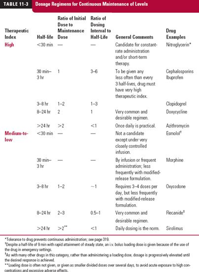
HALF-LIVES BETWEEN 30 MINUTES AND 8 HOURS

For such drugs, the major considerations are therapeutic index and convenience of dosing. A drug with a high therapeutic index need only be administered once every one to three half-lives, or even less frequently. An example is the nonsteroidal anti-inflammatory drug ibuprofen; it has a half-life of around 2 hr, but dosing once every 6 hr, or even 8 hr, is adequate for effective treatment of various inflammatory conditions. A drug with a relatively low therapeutic index must be given approximately every half-life, or more frequently, or be given by infusion. Theophylline, for example, with a half-life of 6 to 8 hr, would need to be given from 3 to 4 times a day; more convenient dosing is achieved by slowing the release of drug from the dosage form (see Modified-Release Dosage Forms discussed on page 311).

HALF-LIVES BETWEEN 8 AND 24 HOURS

Here, the most convenient and desirable regimen is one in which a dose is given every half-life. If immediate achievement of steady state is desired, then, as previously mentioned, the initial dose must be twice the maintenance dose; the minimum and maximum amounts in the body are equivalent to one and two maintenance doses, respectively.

HALF-LIVES GREATER THAN 24 HOURS

For drugs with half-lives greater than 1 day, administration once daily is common, convenient, and promotes patient adherence to the prescribed regimen. For some drugs with very long half-lives, in the order of weeks or more, and which have a moderate to relatively high therapeutic index, once weekly administration is adequate. Examples are mefloquine (half-life of 3 weeks), used as a prophylaxis against malaria, and alendronate, a bisphosphonate (retained and very slowly released from bone, half-life in years) used in the treatment of osteoporosis.

If an immediate therapeutic effect is desired, a therapeutic loading dose needs to be given initially. Otherwise, the initial and maintenance doses are the same, in which case several doses may be necessary before the drug accumulates to therapeutic levels. The decision whether or not to give larger initial doses is often a practical matter. Side effects to large oral doses (gastrointestinal side effects) or to acutely high concentrations of drug in the body may dictate against the use of a loading dose. This is particularly so when, as in many situations, tolerance develops to the adverse effects of a drug (see “Development of Tolerance,” later in this chapter, for further discussion).

REINFORCING THE PRINCIPLES

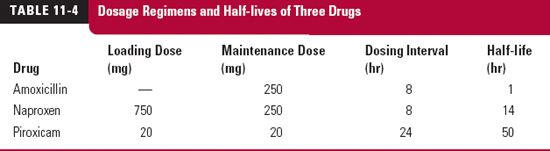
To summarize the foregoing discussion, consider the recommended maintenance dosage regimens given in Table. 11-4 for three drugs. The antibiotic amoxicillin, used to treat an infection, the anti-inflammatory agent, naproxen, when used to treat an acute attack of gout, and piroxicam, another anti-inflammatory agent, when used to treat arthritic joint pain. Listed in Table. 11-5 are the corresponding fractions of the initial amounts remaining at the end of a dosing interval, the average amounts at steady state, and the maximum and minimum values. Instantaneous and complete absorption is assumed, which are reasonable approximations for these drugs.

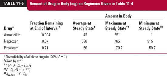
The maintenance doses of amoxicillin and naproxen are the same, but the amounts of them in the body with time at steady state are not. Also, despite the difference in dosage regimens, the average amount in the body at plateau is not that different for amoxicillin and piroxicam. The explanation is readily visualized with a sketch.

For naproxen, the amount in the body immediately after the first dose is 250 mg. At the end of the 8-hr dosing interval, with a half-life of 14 hr, the fraction remaining is 0.67, and the amount therefore is 168 mg. The second maintenance dose of 250 mg raises the amount to 418 mg, and so on. Figure 11-5, curve A, is thus readily drawn, from which it is clear that it takes approximately 3 days to reach steady state, when the average amount in the body is 630 mg (Eq. 11-7), and that the accumulation index is 3.06 (Eq. 11-10). Sometimes, a full therapeutic effect needs to be established more quickly, in which case a loading dose of 750 mg is administered. As can readily be seen, following the loading dose, the amount remaining at the end of the first dosing interval is 505 mg (0.67 × 750 mg), and that the amount lost is 245 mg. The maintenance dose of 250 mg then essentially replaces that lost within this first dosing interval, thereby ensuring that steady-state conditions are maintained throughout the regimen (see colored curve of Fig. 11-5).

For amoxicillin, with a half-life of 1 hr and when 250 mg is given every 8 hr, virtually none remains at the end of the dosing interval (eight half-lives), such that a steady state is reached by the time that the second dose is administered. Events in each dosing interval essentially repeat that following the first dose, fluctuation between maximum and minimum amounts is very large, and in contrast to naproxen, for the same dosage regimen, the average amount within a dosing interval at plateau is only 45 mg (A_av,ss/Dose = 2.5 for naproxen and 0.18 for amoxicillin; Eq. 11-7). Figure 11-6 is a sketch of the amounts of amoxicillin in the body with time.

The results are markedly different for piroxicam than amoxicillin. At the end of each 1-day dosing interval, with a half-life of 50 hr, the fraction remaining for piroxicam is 0.712.

Stay updated, free articles. Join our Telegram channel

Join