(1)
Nanobiophysics Group, University of Twente, Enschede, The Netherlands
Abstract
Multimodal fluorescence imaging is a versatile method that has a wide application range from biological studies to materials science. Typical observables in multimodal fluorescence imaging are intensity, lifetime, excitation, and emission spectra which are recorded at chosen locations at the sample. This chapter describes how to build instrumentation that allows for multimodal fluorescence imaging and explains data analysis procedures for the observables.
Key words
FluorescenceLifetimeExcitationEmissionSpectroscopyMultimodal imagingSupercontinuum light sourceTime-correlated single photon counting1 Introduction
Fluorescence is characterized by the absorption of light, followed by spontaneous emission of light that is typically “red-shifted.” The red-shifted light can be easily separated from the illumination light by choosing a suitable filter set. In fluorescence microscopy, this spectral separation of absorbed and emitted light is exploited to highlight and study specific domains spatially, rendered visible against a dark background. Nevertheless, these methods are of limited use in their ability to analyze the dynamics, interactions, and physical environment of molecules when unassisted by spectroscopy. Imaging spectroscopy methods enable the extension of simple spatial analyses to demonstrate function, co-localization, and molecular interaction at the nanoscale [1].
Multimodal imaging spectroscopy combines imaging with a range of spectroscopic observables to image macro- and microscopic objects, while at the same time obtaining detailed physicochemical information at the micro- and nanoscale. The parameters that are typically measured are fluorescence intensity, lifetime [2], polarization [3], and emission spectra [4]. At the moment, there is an increasing interest in supercontinuum (SC) white light sources [5–7]. These light sources provide the flexibility to pick any desired excitation wavelength between 400 nm and >2,000 nm and allow for time-correlated single photon counting (TCSPC) experiments to accurately measure fluorescence lifetime. Even more important is that SC light sources give the possibility to perform excitation spectroscopy [5, 6, 8], in addition to the commonly measured observables in multimodal microscopy mentioned above. In this chapter, we describe how to assemble and operate a versatile hyperspectral fluorescence lifetime imaging microscopy (FLIM) setup and discuss important practical bottlenecks that are crucial for optimum functionality of the setup.
2 Assembly Procedure
There are many ways to implement multimodal imaging spectroscopy. This chapter describes how to build instrumentation that is capable of both wide-field fluorescence imaging and single-emitter confocal imaging spectroscopy, although the latter method will be the main focus of this chapter. The instrumentation incorporates a supercontinuum white light laser in combination with an acousto-optical tunable filter (AOTF) to provide any desired excitation wavelength in the range between 400 nm and 2,000 nm and allows for fast switching between different wavelengths within the full visible range. The confocal detectors have a sensitivity that is capable of detecting single photons, which not only provides a high signal-to-background ratio but also allows one to study single emitting fluorophores (quantum emitters). The complete setup scheme for the multimodal fluorescence lifetime imaging setup is shown in Fig. 1. This section describes how to assemble each segment and also contains a list of the key components that are needed during each assembly step. Trivial components such as optical mounts, screws, and other minor accessories are not mentioned in these lists but should be included accordingly for the listed modules. The majority of the components used during the assembly of this setup were ordered at Thorlabs Inc. (Dachau/München, Germany). The remaining parts are from different manufacturers and are italicized in the equipment lists.
Fig. 1
Schematic overview of the multimodal fluorescence imaging setup. The parts that are highlighted in red are parts that are essential for the confocal illumination and detection configuration. Without these highlighted components, the setup would operate in conventional fluorescence wide-field imaging configuration. Adding the highlighted components will not degrade the performance in the wide-field imaging configuration. A wide-field illumination source is depicted in this figure for the conventional transmission illumination, but the same light source can be used as well to provide epi-illumination (shaded) through the same light path as the confocal illumination, when focused on the back focal plane of the imaging microscope objective. Filters should be added to this scheme to spectrally separate excitation and emission light. Excitation filters should be placed after the excitation source (wide-field illumination or confocal illumination), and the emission filters should be placed after the wedge
2.1 Microscope Body
The microscope body acts as a solid platform that holds the sample and controls the pathways of light, including the movement of the imaging microscope objective to focus light onto the sample. A convenient configuration is achieved by illuminating the sample through the back-port of the microscope and detecting through one of the other ports. For optimal stability and flexibility, see Note 1.
Olympus IX71 body.
Base stage plate (IX2-SP), to mount the sample holder and piezo stage.
Binoculars (U-BI90).
2.2 Excitation Sources
2.2.1 Wide-Field Illumination
Wide-field illumination can be achieved either by standard transmission illumination by a light source mounted on the illumination pillar above the sample stage or in an epi-illumination configuration through the back-port of the microscope. This combination enables work with transparent as well as nontransparent substrates or samples. The goal of the alignment procedure is to create a homogeneous and intense illumination pattern across the full field of view. Köhler illumination is a commonly used illumination scheme in light microscopy to achieve such illumination and is usually not considered as a critical alignment step. For both high light intensity and good applicability for fluorescence, it is recommended to use high-power LEDs or a Mercury lamp (see Note 2).
Illumination pillar, condenser.
M470L2-C1: High-power blue LED with collimator and adapter for Olympus BX/IX (additional power LEDs are available as well for UV, VIS, and NIR spectral ranges).
DC2100: High-power LED driver—1–100 kHz modulation option.
(Optional) Olympus 100 W Mercury Lamp.
2.2.2 Confocal Illumination
Coupling Light into the Single-Mode Fiber
Before the confocal illumination path can be aligned, the light from the SC400-PP supercontinuum excitation source must be coupled into a single-mode fiber to spatially clean up the excitation light and provide a Gaussian illumination profile from a point source at the other end of the fiber. Use a kinematic mirror mount to fix the collimator of the supercontinuum laser and couple the collimated white light beam through the acousto-optical tunable filter (AOTF) with a precision of ±0.5° with respect to the normal of the AOTF crystal (caution, high radiation, do not use full power for alignment). This AOTF crystal diffracts only a small spectral band by applying a fixed radio-frequency (RF) signal and blocks remaining unwanted wavelengths. Use the manufacturer’s software to open a channel of the AOTF to transmit a narrow band of visible light at the back-end of the AOTF. Three different beams can be seen at the back: the zeroth order (white light), which should be blocked with a proper beam block, and two first-order diffracted beams (well-defined bands). Only one of the first-order beams is collinear with the crystal and does not displace when the AOTF is tuned to a different wavelength. This collinear beam needs to be coupled into a single-mode fiber (P1-460A) using two mirrors, incoupling optics (A240TM-A), and a precision XYZ stage (MBT613D/M).
Supercontinuum white light source (SC400-PP) from Fianium Ltd. (Southampton,UK).
1 mount for the output fiber of the SC400-PP laser.
Crystal Technologies broadband acousto-optical tunable filter (AOTF) + RF controller.
1 rotation stage for the AOTF.
1 beam block to block stray light and unwanted orders from the AOTF.
2 broadband visible light mirrors + 2 kinematic mirror mounts.
A240TM-A aspheric lens, f = 8 mm + E12RMS adapter.
MBT613D/M 3-axis precision fiber incoupling platform.
P1-460A single-mode optical fiber.
Acousto-optical Tunable Filter Calibration
The calibration of the AOTF allows one to choose any desired excitation wavelength and opens up possibilities for excitation spectroscopy and hyperspectral imaging. Calibration of the AOTF is done by applying different RF frequencies to the crystal and measuring the corresponding transmission wavelengths using a calibrated spectrograph (CCS100/M). The peak transmission wavelength as a function of RF frequency is the required calibration curve and should be fitted with a cubic polynomial fit. The corresponding polynomial coefficients are used in custom written software to convert the desired wavelength to the RF frequency that has to be applied to the crystal.
CCS100 USB spectrograph
Collimation of the Excitation Beam
The best confocal illumination spot is achieved by projecting a small point source (single-mode fiber exit) into a small diffraction-limited illumination focus spot at the sample plane. Before the light enters the infinity-corrected imaging microscope objective, the light should be collimated, and its beam diameter should roughly match the back aperture of the imaging objective. The infinity-corrected RMS4X collimation objective can be used to collimate the light coming out of the single-mode fiber (NA 0.1) and slightly overfill the back aperture, which produces the sharpest confocal illumination spot (for more details, see Note 3).
MBT616D/M 3-axis precision stage.
1 kinematic mirror mount for XY tilt angles + FC connector adapter to mount the fiber.
RMS4X objective to collimate the output light.
1 SM1-RMS external-internal ring adapter and 1 thick 30 mm cage plate to mount the RMS4X objective.
500 mm telescope to accurately collimate laser light (Möller-Wedel FR500/65/14.7).
Aligning the Excitation Beam to the Central Optical Axis
After collimating the excitation beam, the excitation beam needs to be aligned to the central optical axis of the imaging objective. First, place the mirrors on a breadboard at the same height as the back-entrance of the microscope. Position two mirrors which are mounted in robust gimbal mounts such that the excitation beam is directed in a Z-angled configuration and reflected by the wedge along the central optical axis of the imaging objective (see Note 4).
2 gimbal mirror mounts + 2 mirrors.
Beam splitter: BSF10-A—beam sampler, which deflects the ghost beam.
2.3 Detection Path
2.3.1 Imaging CCD
The imaging CCD is used to obtain a picture of a full area at one instance. A good test sample to align the CCD would be a standard microscopy test sample of the plant Convallaria majalis (Lily of the valley, Fig. 2), because it is highly autofluorescent and shows a large spectral diversity. Illuminate the Convallaria sample using the wide-field illumination source and sharply focus the sample using the microscope’s binoculars. Direct the fluorescence emission light towards the CCD and focus the fluorescence emission light onto the CCD. Be sure to use the proper filters to spectrally separate the excitation light (typically, a band-pass filter) and emission light (typically, a long-pass filter).
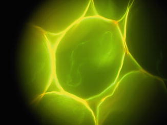
Fig. 2
Wide-field fluorescence image of Convallaria majalis (Lily of the valley). Lifetime and spectral data can be recorded once the confocal detectors have been aligned (Fig. 4)
Test sample: Convallaria majalis (Lily of the valley).
Imaging lens (180 mm ø2 inch achromat, or tube lens of the microscope).
CMOS or CCD camera (Zeiss Axiocam or Andor iXon3).
Filters, for example: FF02-447/60 band-pass for the excitation light and BLP488R long-pass for the emission light (same filters can be used for the confocal fluorescence microscopy configuration).
2.3.2 Confocal Detectors
The confocal detector acts as a point detector, which measures fluorescence emission from a well-defined volume. To constrain the detection to this volume, it is necessary to remove as much stray light as possible (see Note 5). After proper shielding, the dark noise level should match the specified level given by the manufacturer of the detector. Since the confocal detection volume is static, the sample has to be raster-scanned through this detection volume to record intensity and lifetime (avalanche photodiode) and emission spectra (spectrograph) at each point. The incorporation of the scanning stage into the confocal detection scheme is explained at the end of this section.
Stay updated, free articles. Join our Telegram channel

Full access? Get Clinical Tree


