Table 8.1 shows that in one year a prestigious university admitted 52% of male applicants compared with only 45% of female applicants, suggesting that there was a bias in favour of men. When quizzed about this, the two main faculty heads said that it couldn’t be true, they had both admitted a higher proportion of women than men: the success rate in arts was 38% for women and only 32% for men and that in science was 66% for women compared with only 62% for men. How can this be?
| Faculty | Men | Women | ||||
|---|---|---|---|---|---|---|
| Applicants | Admitted | Percentage | Applicants | Admitted | Percentage | |
| Arts | 4,100 | 1,300 | 32 | 8,250 | 3,150 | 38 |
| Science | 8,200 | 5,100 | 62 | 2,900 | 1,900 | 66 |
| Total | 12,300 | 6,400 | 52 | 11,150 | 5,050 | 45 |
This is an example of Simpson’s paradox, an extreme form of confounding where an apparent association observed in a study is in the opposite direction to the true association. In this example it arose because women were much more likely to apply to arts courses, for which applicants had a lower overall success rate.
In Chapters 6 and 7 we considered two reasons why the results of a study might not be the truth, namely chance and error or bias. In this chapter we will consider a third possible ‘alternative explanation’ – confounding.
Confounding refers to a mixing or muddling of effects that can occur when the relationship we are interested in is confused by the effect of something else. It arises when the groups we are comparing are not completely exchangeable and so differ by factors other than their exposure status (whether they are ‘exposed’ or ‘not exposed’). If one (or more) of these other factors is a cause of both the exposure and the outcome, then some or all of an observed association between the exposure and outcome may be due to that factor. For example, if in a cohort study we observe that people with yellow fingers have a higher incidence of lung cancer compared to those who do not have yellow fingers, does this mean that having yellow fingers causes you to get lung cancer? Of course, the reason we see this association is because the exposure ‘yellow fingers’ and the outcome ‘lung cancer’ share a common cause – tobacco smoking (Figure 8.1). The exposure groups we are comparing (those with and without yellow fingers) are therefore not exchangeable because people with yellow fingers are more likely to be smokers than people who do not have yellow fingers. As a result, they are also more likely to get lung cancer. Even if an exposure does not cause a disease, it will appear to be associated with the disease if both it and the disease are caused by a third factor, in this case smoking. The relation between yellow fingers and lung cancer is therefore confounded by smoking.
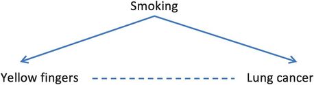
The relation between smoking, yellow fingers and lung cancer.
Confounding can be a major problem and has to be addressed in all non-randomised research and in some randomised trials as well, especially if they are small. As in previous chapters, we will mainly discuss confounding in the context of studies of the causes of a disease but, as with all epidemiological methods, everything that we say will apply equally to any study looking at associations.
The following hypothetical case–control study of alcohol and lung cancer illustrates how easily confounding can arise and how it can be diagnosed. It also suggests how confounding can be dealt with and we will discuss this in more detail later in the chapter.
An example of confounding: is alcohol a risk factor for lung cancer?
Imagine a (very small) case–control study with 20 cases (people with lung cancer ☹) and 20 controls who do not have lung cancer (☺). Is drinking alcohol associated with the risk of lung cancer? If all the cases and controls were asked about their alcohol consumption we could classify people as ‘drinkers’ (☹,☺) or ‘non-drinkers’ (☹,☺) (Figure 8.2) and calculate an odds ratio to estimate the strength of the association between alcohol and lung cancer.
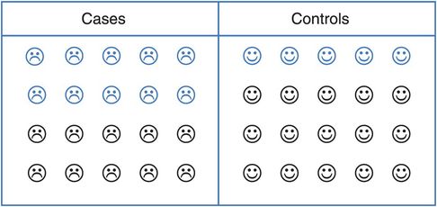
A hypothetical case–control study of alcohol and lung cancer (blue = drinkers, black = non-drinkers).
What is the odds ratio for the association between alcohol and lung cancer?
Can we conclude that alcohol consumption is associated with lung cancer?
As Table 8.2 shows, the odds ratio for the association between alcohol and lung cancer is 3.0, suggesting that the risk of developing lung cancer in people who drink alcohol is three times that in non-drinkers.
| Cases | Controls | ||
|---|---|---|---|
| Alcohol drinkers | 10 | 5 | 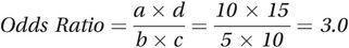 |
| Non-drinkers | 10 | 15 |
However, we know that smokers are much more likely to develop lung cancer than non-smokers, and it is possible that they are also more likely to drink alcohol than non-smokers. Could smoking have affected the association we saw between alcohol and lung cancer? To investigate this we need to separate the smokers from the non-smokers and look at the association between alcohol and lung cancer – the ‘alcohol effect’ – in each group. Figure 8.3 shows that 12 of the 16 smokers were also alcohol drinkers compared with only 3 of the 24 non-smokers.
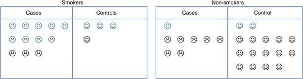
Separating smokers and non-smokers (blue = drinkers, black = non-drinkers).
Calculate the odds ratio for alcohol and lung cancer separately for (i) smokers and (ii) non-smokers. (Hint: first draw up the appropriate 2 x 2 tables.)
Is alcohol associated with lung cancer among smokers? Among non-smokers?
How do you explain the change in the pattern of the alcohol–lung cancer relationship?
The odds ratio for the association between alcohol and lung cancer among smokers is 1.0. Fewer of the non-smokers drink alcohol, but again the odds ratio is 1.0 (see Table 8.3). This process in which we divide or stratify the study participants into two or more separate groups (strata) is known as stratification.
| Cases | Controls | |||
|---|---|---|---|---|
| Smokers | Alcohol drinkers | 9 | 3 | 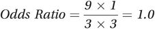 |
| Non-drinkers | 3 | 1 | ||
| Non-smokers | Alcohol drinkers | 1 | 2 | 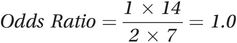 |
| Non-drinkers | 7 | 14 |
So, although there appears to be an association between alcohol and lung cancer in the whole study population, it disappears when we consider smokers and non-smokers separately. We could then go on to combine the odds ratios in smokers and non-smokers to calculate a pooled odds ratio that is adjusted for the effects of smoking. In this example, the adjusted odds ratio is also 1.0. (We will not discuss the methods for calculating an adjusted odds ratio here, but a common method, developed by Mantel and Haenszel (1959), is shown in Appendix 8.)
The apparent (crude) overall relationship we saw between alcohol and lung cancer arose because while those with lung cancer were indeed more likely to drink alcohol than those without lung cancer, alcohol and smoking go together so they were also more likely to be smokers than those without lung cancer. The increased risk of lung cancer among alcohol drinkers was in fact due entirely to their smoking.
This situation, in which an apparent relationship between an exposure and an outcome is really due, in whole or in part, to a third factor that is associated both with the exposure and with the outcome of interest is known as confounding. In the example, smoking is said to be a confounder of the alcohol–lung cancer link. Confounding is a mixing of effects because the effect of the exposure we are interested in (e.g. alcohol) is mixed up with the effect of some other factor (e.g. smoking). To look at the real effect of the exposure we have to first deal with the effect of the confounder.
Characteristics of a confounder
As you saw above, a confounder is a factor that is associated with both the exposure and the outcome. Strictly speaking, these associations should be causal as in the yellow fingers example at the start of the chapter – smoking causes both yellow fingers and lung cancer. However, in practice the confounder may just be a proxy for the true cause and this is the situation in the smoking and alcohol example. Smoking does not cause someone to drink alcohol in the usual sense of the word, but instead both behaviours probably result from a complex interplay of genes, socioeconomic status (SES) and environment. Importantly, the confounder must not be a consequence of either the exposure or the outcome. So, to summarise, for something to be a confounder it must:
be a risk factor for disease (among those who are not exposed to the factor of interest),
be associated with the exposure of interest (in the source population or among the controls in a case–control study) and
not be an intermediary between exposure and the outcome (i.e. it must not lie on the causal pathway).
Look back to Figure 8.3 and check that smoking has these attributes in the alcohol and lung cancer example.
Among non-drinkers what proportion of (i) cases and (ii) controls smoked?
Among the controls what proportion of (i) smokers and (ii) non-smokers drank alcohol?
Is alcohol likely to cause smoking? (That is, could smoking lie on a causal pathway between alcohol and lung cancer?)
In the alcohol example, smoking was a confounder for the following reasons.
(1) It was associated with lung cancer: among people who did not drink alcohol, 3 out of 10 cases were smokers (30%) compared with only 1 of 15 controls (7%). That is, among non-drinkers, the cases were more likely to smoke than were the controls.
(2) It was associated with alcohol among the controls: 3 out of 4 controls who smoked also drank alcohol (75%), compared with only 2 out of 16 controls who did not smoke (12.5%). That is, among the controls, smokers were more likely to drink alcohol than were non-smokers.
(3) It is not on a causal pathway between alcohol and lung cancer: although alcohol and smoking often go together, drinking alcohol does not ‘cause’ someone to be a smoker.
An example of an intermediary is seen in the association between obesity and heart disease. High blood pressure is related both to obesity (the exposure) and to heart disease (outcome) and could, therefore, be a potential confounder of this association. However, because raising blood pressure is part of the causal path through which obesity acts to increase the risk of heart disease (obesity → increased blood pressure → heart disease), it would be misleading to adjust for this, as it would remove part of a real causal effect of being heavy.
Figure 8.1 illustrates these criteria, showing how when a confounder is causally related both to the exposure and to the outcome of interest, the exposure may appear to be related to the disease even when it is not. Because having yellow fingers is associated with (caused by) smoking and smoking causes lung cancer, yellow fingers and lung cancer appear to be associated. Figure 8.1 is an example of a directed acyclic graph or DAG. DAGs are a very helpful way to visualise the relationships among the different factors that might affect an outcome and also to identify potential confounding variables (see Box 8.2 for more information about DAGs). We could also draw a DAG for the alcohol and lung cancer example but, as we noted above, while tobacco smoking clearly causes lung cancer, it is not so obviously a ‘cause’ of alcohol consumption. In practice, it is likely that tobacco smoking is a proxy for some unmeasured factor or factors (designated ‘U’) that are a common cause of both smoking and alcohol consumption and this is illustrated in Figure 8.4. In this example, smoking fulfils the criteria for a confounder because alcohol is associated with smoking (because they share the common cause U) and smoking is associated with lung cancer.
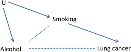
A DAG showing how smoking confounds the relation between alcohol and lung cancer.
The effects of confounding
In the example above, the apparent effect of alcohol on lung cancer was entirely due to the effect of smoking, but confounding does not necessarily create an apparent effect where really there is none. Confounding can lead to either overestimation or underestimation of the size of a real effect, it can completely hide a real association that exists and in very extreme situations it can even reverse the direction of an effect, making it appear that a cause of a disease actually protects against it. (This is known as Simpson’s paradox and it explains the apparent contradiction in the university admissions data at the start of the chapter).
Age, sex and SES are common confounders. As an example, many diseases occur more frequently in older people. If the exposure of interest also occurs more commonly in the elderly, e.g. a poor diet, then the confounding effects of age would have to be considered.
Authors of early studies that looked at the relation between diet and heart disease found that the more a person ate, the lower their risk of heart disease. This apparent association was all the more surprising because we know that obesity is a risk factor for heart disease. However, one factor that the studies did not take into account was physical activity and, on average, people who are physically active eat more than those who are inactive, i.e. physical activity is potentially a cause of high energy intake and physical activity also reduces risk of heart of disease. Could this have affected the results of the studies?
Table 8.4 presents the results of a hypothetical case–control study evaluating the association between energy intake and heart disease.
| Energy intake | Total | High physical activity | Low physical activity | |||
|---|---|---|---|---|---|---|
| Heart disease | Controls | Heart disease | Controls | Heart disease | Controls | |
| High | 730 | 600 | 520 | 510 | 210 | 90 |
| Low | 700 | 540 | 100 | 150 | 600 | 390 |
Is physical activity associated with energy intake in this study?
Draw a DAG showing the likely relationships between energy intake, physical activity and heart disease.
Is physical activity likely to confound the relationship between high energy intake and heart disease? Why?
Table 8.4 clearly shows that people who are more active consume more energy than those who are less active (510 ÷ 660 = 77% of active controls have high energy intake compared to only 90 ÷ 480 = 19% of inactive controls). Figure 8.5 shows a DAG for this example, suggesting that physical activity is a common cause of both energy intake and heart disease and so is likely to confound the association between them.
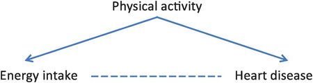
A DAG showing how physical activity will confound the relation between energy intake and heart disease.
What is the odds ratio for the crude association between high energy intake and heart disease?
What is the odds ratio for the association between high energy intake and heart disease in people with (i) high and (ii) low levels of physical activity?
Is the association between high energy intake and heart disease confounded by the level of physical activity?
The crude odds ratio for the association between high energy intake and heart disease in this study is (730 × 540) ÷ (700 × 600) = 0.9, i.e. those with high energy intake appear to have a 10% lower risk of coronary heart disease (CHD). When we stratify by physical activity the odds ratio is (520 × 150) ÷ (100 × 510) = 1.5 among the physically active and (210 × 390) ÷ (600 × 90) = 1.5 among the inactive. Thus, when we remove the confounding effects of physical activity by stratification, high energy intake is associated with a 50% higher risk of CHD (OR = 1.5). In this example the confounding meant that the observed odds ratio (OR = 0.9) was an underestimate of the true association between obesity and CHD (OR = 1.5).
Although this example was a case–control study, confounding can occur in exactly the same way in a cohort study (see the questions at the end of the chapter for an example of this).
How can we tell if an association is confounded?
If a factor has the characteristics of a confounder (see above) and when you stratify or adjust for it the effect estimate changes, then confounding is present. In the lung cancer example at the start of the chapter the odds ratio dropped from 3.0 to 1.0 when we adjusted for smoking, indicating that smoking was a strong confounder. In the heart disease example the estimate increased from 0.9 to 1.5 when we adjusted for physical activity, so again this was confounding the association. A commonly used rule is that if, when you adjust for a potential confounder, the crude and adjusted effect estimates differ by 10% or more, then the crude estimate is confounded to some degree and it is more appropriate to present the adjusted value.
When will a possible confounder actually be a confounder in practice?
There are many things that could confound an association between an exposure and outcome, but in practice they might not actually do so.
Table 8.5 shows the characteristics of a group of women at the time of recruitment into a cohort study of oral contraceptives (OCs) and CHD.
| Oral contraceptive use | ||
|---|---|---|
| Yes | No | |
| Percentage aged less than 30 years | 60 | 30 |
| Percentage of low SES | 50 | 40 |
| Percentage smoking >15 cigarettes/day | 17 | 12 |
| Mean body mass index (weight (kg)/height (m)2) | 26.5 | 27.0 |
| Percentage with a history of: | ||
| Hypertension | 1 | 1 |
| Stroke | 0.03 | 0.3 |
| Venous thromboembolism | 1 | 8 |
Assume that all the factors are known risk factors for CHD. Which of them might be confounders of the OC–CHD relationship? Why?
For something to be a confounder it has to be associated both with the exposure of interest (OC use) and with the outcome of interest (CHD). All of the factors listed are known risk factors for CHD, so they are all associated with CHD. Some are also associated with OC use – we can see from Table 8.5 that, compared with non-users, OC users are:
twice as likely to be under the age of 30 as non-users (60% versus 30%),
slightly more likely to be of low SES (50% versus 40%),
slightly more likely to be current smokers (17% versus 12%),
10 times less likely to have had a stroke (0.03% versus 0.3%) and
8 times less likely to have had a venous thromboembolism (1% versus 8%).
So will these factors confound the association between OC use and CHD?
In practice, it turns out that only age, history of thromboembolism and, to a lesser extent, smoking are likely to affect the results appreciably. Because CHD rates increase with age, the rate in the OC users will be lower than in the non-users simply because they are younger. If OC use truly increased the risk of CHD, say the true RR = 3.0, then the effect of confounding by age might reduce the observed RR (unadjusted for age) to about 2.5 (Table 8.6), thus reducing the (real) difference between the groups. Similarly, the eightfold difference between the OC users and non-users in terms of their history of thromboembolism, a strong risk factor for CHD, will also bias the observed RR downwards to about 2.4. Conversely, CHD rates are higher in smokers and OC users are slightly more likely to be smokers than non-users, thus the effect of confounding by smoking would be to increase the apparent RR, making the effect look stronger than it really is.
| Oral contraceptive use | Likely | ||
|---|---|---|---|
| Yes | No | Observed RRa | |
| Percentage aged less than 30 years | 60 | 30 | 2.5 |
| Percentage of low SES | 50 | 40 | 3.2 |
| Percentage smoking >15 cig/day | 17 | 12 | 3.3 |
| Mean body mass index (weight (kg)/height (m)2) | 26.5 | 27.0 | 2.9 |
| Percentage with a history of: | |||
| Hypertension | 1 | 1 | 3.0 |
| Stroke | 0.03 | 0.3 | 2.9 |
| Venous thromboembolism | 1 | 8 | 2.4 |
a Estimated RR for OC use and CHD, assuming that the RRs for the associations between the potential confounders and CHD are: 2.0 for age, 2.0 for SES, 4.0 for smoking, 4.0 for BMI, 10.0 for stroke and 5.0 for venous thromboembolism.
This contrasts strikingly with the confounding influence of a history of stroke. Theoretically this looks sure to be an important confounder, given the 10-fold difference between OC users and non-users in terms of their past stroke experience, i.e. a very strong association between OC use and stroke (note that this occurs because women who have had a stroke would not normally be prescribed the OC pill), and the very strong known link between stroke and heart disease (due to their common set of risk factors). However, because stroke is so rare in young women, this imbalance affects only a tiny proportion of the total study group, and so has a trivial effect on the crude RR, biasing it downwards by <5%, from 3.0 to 2.9. Even if a history of stroke had been five times more common in the study groups (0.015% and 1.5%), the RR would have been biased downwards by only about 10%, from 3.0 to 2.7. More predictably, strong independent risk factors for CHD such as low SES and BMI also fail to confound when their distributions in the groups being compared are reasonably similar, i.e. the groups are still exchangeable with respect to these factors. So for something to be a confounder in practice it must not only be associated quite strongly with the exposure and the outcome, it must also be reasonably prevalent in the population.
As another example, consider the case–control study of energy intake and heart disease shown in Table 8.4. In this study the prevalence of the confounder (physical activity) in the population was very high – 660 of the 1140 controls or 58% were physically active. What would have happened to our analysis if the population had been much less active? Table 8.7 shows results from a similar study for a population in which only 6% of controls were physically active. (To obtain these numbers we have just divided the numbers in the physically active group by 10 and multiplied the numbers in the inactive group by 2.) The stratum-specific odds ratios, and thus the adjusted odds ratio, are unaffected but the crude odds ratio is now 1.3 instead of 0.9; i.e. it is much closer to the unconfounded value of 1.5 and there is much less confounding by physical activity because this is now much less common.
| Energy intake | Total | High physical activity | Low physical activity | |||
|---|---|---|---|---|---|---|
| Heart disease | Controls | Heart disease | Controls | Heart disease | Controls | |
| High | 472 | 231 | 52 | 51 | 420 | 180 |
| Low | 1210 | 795 | 10 | 15 | 1200 | 780 |
| OR | 1.3 | 1.5 | 1.5 | |||
Stay updated, free articles. Join our Telegram channel

Full access? Get Clinical Tree


