and our alternative hypothesis is simply:

Now, if we were to set about comparing the means5 with a t-test, a problem would arise. We can do only two at a time, so we end up comparing R with S, R with T, R with U, S with T, S with U, and T with U. There are 6 possible comparisons, each of which has a .05 chance of being significant by chance, so the overall chance of a significant result, even when no difference exists, approaches .30.6 In any case, we really don’t care about the specific differences in the first round.
This is where the complicated formula comes in. Thinking in terms of signals and noises, what we need is a measure of the overall difference among the means of the groups and a second measure of the overall variability within the groups. We approach this by first determining the sum of all the squared differences between group means and the overall mean. Then we determine a second sum of all the squared differences between the individual data and their group mean. These are then massaged into a statistical test.
THE PARTS OF THE ANALYSIS
Sums of Squares
With the t-test, our measure of the signal was the difference between the means. As we just saw, though, we can’t do that when we have more than two groups, so what do we use? Another way of thinking about what we did with the t-test was that we got the grand mean of the two groups (which we abbreviate as  .. for reasons we’ll explain shortly), and then saw how much each individual mean deviated from it:

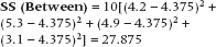
We use the same logic with the analysis of variance (ANOVA); we figure out the grand mean of all of the groups, and see how much each group mean deviates from it. As we saw when we were deriving the formula for the SD in Chapter 3, though, this will always add up to zero, unless we square the results. We also need to take into account how many subjects there are in each group. We call the results the Sum of Squares (Between), because it is literally the sum of the squared differences between the group means and the grand mean. So what we have is:

where n is the number of subjects in each group. If the groups have different sample sizes, you would use the harmonic mean of the sample sizes, as explained in Chapter 3.
Time to explain those funny dot subscripts. Each person’s score is represented as X. Now, we need some way of differentiating Subject 1’s score from Subject 2’s, and so on, so we have one subscript (i) to indicate which subject we’re talking about. But, we in essence have four Subject 1s—one from each of the groups, so we need another subscript (k) to reflect group membership. A dot replacing a subscript means that we’re talking about all of the people referred to by that subscript. So,  is the mean of all people in Group k, and
  .. is the mean of all people in all groups (i.e., the grand mean).
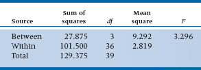
Let’s just fake up some sex satisfaction data7 to illustrate what we did, and these are shown in Table 8–1. Using Equation 8–4, we’ll get:
Similarly, the Sum of Squares (Within) is the sum of all the squared differences between individual data and the group mean within each group. It looks like:
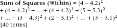
After much anguish, this turns out to equal 101.50. Again, the algebraic formula, for the masochists in the crowd, is:

where the first summation sign, the one with the i under it, means to add over all of the subjects in the group, and the second summation sign means to add across all the groups.
Finally, the Sum of Squares (Total) is the difference between all the individual data and the grand mean. It is the sum of SS (Between) and SS (Within). But in longhand:
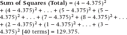
TABLE 8–1 Satisfaction ratings with 4 brands of condoms, 10 subjects each
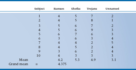
Based on a 10-point scale where 1 is the pits and 10 is ecstasy.
To check the result, this should be equal to the sum of the Between and Within Sums of Squares, 27.875 + 101.50 = 129.375; and the algebraic formula is:

There are two things to note. First, because summation is usually obvious from the equation, from now on, we’ll just use a single Σ without a subscript, even when two or more are called for, and let you work things out. Second, the equations look a little bit different if there aren’t the same number of subjects in each group, but we’ll let the computer worry about that wrinkle.
Degrees of Freedom
The next step is to figure out the degrees of freedom (df or df or d.f.) for each term, preparatory to calculating the Mean Squares. Remember that in the previous chapter, we defined df as the number of unique bits of information. For the Between-Groups Sum of Squares, there are four groups, whose sum must equal the Grand Mean. So, the df (Between) is equal to 4 − 1 = 3. More generally, for k groups:

We follow the model for the t-test for the Within-Groups Sum of Squares, where we figured out the df for each group, and then added them together. Here, each of the four groups has 10 data points, so df is 4 × (10 − 1) = 36. In general, then:

Finally, for the Total Sum of Squares, there are 40 data points that again must add up to the Grand Mean, so df = 39. Again, generally, the formula is:

It’s no coincidence that the df for the individual variance components (between and within) add up to the total df. This is always the case, and it provides an easy check in complex designs.
Mean Squares
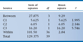
Now we can go the next, and last, steps. First we calculate the Mean Square by dividing each Sum of Squares by its df. This is then a measure of the average deviation of individual values from their respective mean (which is why it’s called a Mean Square), since the df is about the same as the number of terms in the sum. Finally, we form the ratio of the two Mean Squares, the F-ratio, which is a signal-to-noise ratio of the differences between groups to the variation within groups. This is summarized in an ANOVA table such as Table 8–2. We can then look up the calculated F-ratio to see if it is significant.
The critical values of the F-test at the back of the book are listed under the df for both the numerator and the denominator. When you publish this piece (good luck!!), the F-ratio would be written as F3,36 or, if you can’t afford the word processor, F(3,36) or F(3/36). Either way, the calculated ratio turns out to be significant because 3.296 is just a bit greater than the published F-value for 3 and 36 df, 2.86. So Julius may have taken them all out of the same latex vat, but all condoms are not created equal. At this point, we know that at least two are different from each other, but it can’t say yet which they are; we’ll get to that when we discuss post-hoc comparisons.
EXPECTED MEAN SQUARES AND THE DISTRIBUTION OF F
If you peruse the table of F-ratios in the back, one fact becomes clear—you don’t see F-ratios anywhere near zero. Perhaps that’s not a surprise; after all, we didn’t find that any t-values worth talking about were near zero either. But it actually should be a bit more surprising, if you consider where the F-ratio comes from. After all, the numerator is the signal—the difference between the groups—and the denominator is the differences within the groups. If no difference truly exists between the groups, shouldn’t the numerator go to zero?
Surprisingly, no. Imagine8 that there really was no difference among the condoms. All the =s are therefore equal. Would we expect the Sum of Squares (Between) to be zero? As you might have guessed, the answer is “No.” The reason is because whatever variation occurred within the groups as a result of error variance would eventually find its way into the group means, and then in turn into the Sum of Squares (Between) and the Mean Square. As it turns out, in the absence of any difference in population means, the expected Mean Square (Between) [usually abbreviated as E(MSbet)] is exactly equal to the variance (within), σ2err.
TABLE 8–2 The ANOVA summary table
Conversely, if no variance exists within groups, then the only variance contributing to the Mean Square is between groups, and the expected Mean Square (Between) = n × σ2bet.
Putting it together, then, the expected value of the Mean Square (Within) is just the error variance, σ2; and the expected value of the Mean Square (Between) is equal to the sum of the two variances:

So when there is no true variance between groups, the σ2bet drops out and the ratio (the F-ratio) equals 1.
As we go to hairier and hairier designs, the formulae for the expected mean squares will also become hairier (to the extent that this is the last time you will ever see the beast derived exactly), but one thing will always remain true: In the absence of an effect, we expect the relevant F-ratio to equal 1. Conversely, if we go to a really simple design and do a one-way ANOVA on just two groups, the calculated F-ratio is precisely the square of the t-test.
Does this mean that you’ll never see an F-ratio less than 1? Again, the same answer, “No.” Because of sampling error, it sometimes happens that when nothing is going on—there’s no effect of group membership—you’ll end up with an F that’s just below 1. Usually it’s in the high .90s.
ASSUMPTIONS OF ANOVA
One-way ANOVA, as well as the t-test and all other ANOVAs, makes two assumptions about the data. The first is that they are normally distributed, and the second is that there is homogeneity of variance across all of the groups. The first assumption, normality, is rarely tested formally because, as Ferguson and Takane (1989) state, “Unless there is reason to suspect a fairly extreme departure from normality, it is probable that the conclusions drawn from the data using an F-test will not be seriously affected” (p. 262). That is, the Type I and Type II errors aren’t inflated if the data are skewed (especially if the skew is in the same direction for all groups); and deviations in kurtosis (the distribution being flatter or more peaked than the normal curve) affect power only if the sample size is low.
There’s another very good reason not to worry about it. If we go back to Chapter 6 and the logic of statistical inference, what we’re actually looking at with ANOVA, t-tests, and any other statistic focused on differences between means, is the distribution of the means. From the Central Limit Theorem (Chapter 4), the means will be normally distributed, regardless of the original distribution, especially when there are at least 30 or so observations per group.
The assumption of homogeneity of variance, which also goes by the fancy name of homoscedasticity, is assessed more often because most computer programs do it whether we want it or not, but the results are rarely used. The reason is that one-way ANOVA is fairly robust to deviations from homoscedasticity (which is called, for obvious reasons, heteroscedasticity), especially if the groups have equal sample sizes, and the populations (not the samples) are normally distributed. Just how robust is anybody’s guess, but as with the assumption of normality, it’s rarely worth worrying about, especially if the ratio of the largest to the smallest variance is less than 3 (Box, 1954).
MULTIPLE COMPARISONS
One could assume, in the above experiment, that finding the F-ratio concluded the analysis. The alternative hypothesis was supported, the null hypothesis was rejected, and so on. You don’t really care which of the condoms resulted in the most satisfaction—or do you? There are certainly many occasions where one might, out of genuine rather than prurient interest, wish to go further after having rejected the null hypothesis to determine exactly which specific levels of the factor are leading to significant differences.
In fact, situations also occur when, although there may be more than two levels in the analysis, the previous hypothesis can be framed much more precisely than simply, “Not everything is equal.” In the present example, if we were going up against Julius Schmid, our real interest is a comparison of Brand U (unnamed) against the average of brands R, S, and T. More commonly, a comparison of three or four drugs, such as a group of aspirin-based analgesics that includes a placebo, almost automatically implies two levels of interest—all analgesics against the placebo, and, if this works, comparisons among analgesics.
These two situations are described as post-hoc comparisons, occurring out of interest after the primary analysis has rejected the null hypothesis; and planned comparisons, which are deliberately engineered into the study before the conduct of the analysis.
Planned comparisons are hypotheses specified before the analysis commences; post-hoc comparisons are for further exploration of the data after a significant effect has been found.
As you might have guessed, post-hoc comparisons are considered to be more like data-dredging, and thus inferior to the elegance of planned comparisons. However, they are much more common and also easier to understand, so we will start at the end and work forward.
Family-Wise and Experiment-Wise Error Rates
In Chapter 6, we mentioned some of the problems with multiplicity (running many tests of significance). There, we discussed it in the context of doing a number of separate tests, such as looking at baseline differences between groups across a number of variables, examining a large number of correlations, or looking at two or more outcomes. Once we enter the realm of ANOVAs, we add a new level of complexity.9 In the example we’ve just used, we looked at users’ satisfaction ratings of four brands of condoms. But let’s say that the study was actually more complicated than this, and we also wanted to look at the satisfaction of the partner(s), ease of use, and comfort level as dependent variables; and as another independent variable, comparing experienced with novice users (assuming we can find any of the latter). Now we have four DVs and two IVs, so if we want to look at the two experience levels separately (which is all we know how to do at this point), we can be running eight one-way ANOVAs, and each ANOVA can compare Ramses against Sheiks, Ramses against Trojans, and so on, for six possible pairwise comparisons. That’s a lot of F-ratios and t-tests running around (48, to be precise). Do we have to correct for all of them?
Well, let’s first distinguish between family-wise and experiment-wise error rates. By the experiment-wise error rate, we mean all of the hypotheses tested in the experiment (see, that was easy), and there are in fact 48 of them, such as “Is there a difference between Sheiks and Unnamed in terms of ease of use for novices,” “Is there a difference between Ramses and Trojans in terms of user satisfaction for experienced users,” and so on. If we consider all of these hypotheses to be independent, then we would have to correct for the fact that we are testing 48 hypotheses. This will result in a tremendous loss of power, and a high probability of Type II errors. However, some of the tests can be considered to be parts of families of hypotheses; “Is there a difference among brands in terms of pleasure for mavens (or mavonim, if you want to be pedantic about it)?” The post-hoc tests that we will discuss in the next section correct for the family-wise error rate, such that when comparing condom brands for novice users, they recognize that there will be six pair-wise tests. Needless to say, they can’t correct for the experiment-wise error rate, because the computer, bright as it may seem (which is rarely), doesn’t know how many separate analyses you’re going to run. If all of the tests are planned ahead of time (that is, you’re not on a fishing expedition), that’s not a problem. Jaccard and Guilamo-Ramos (2003) recommend correcting for multiplicity within families of tests, but not across them.
POST-HOC COMPARISONS
All the post-hoc procedures we discuss—Fisher’s LSD (Least Significant Difference), Tukey’s HSD (Honestly Significant Difference), the Scheffé Method, the Neuman-Keuls Test, and Dunnett’s t (and a lot more we won’t discuss)—involve two comparisons at a time.
Because we have only a limited number of ways to look at the difference between two means (subtract one from the other and divide by a noise term), they all end up looking a lot like a t-test. All of these tests assume equal variances for the groups (we’ll mention, but not discuss, tests to use when the variances aren’t equal). They differ among themselves in two regards—how they try to control for multiplicity, and whether they are multiple comparison or range tests (some are both). Multiple comparison tests compare each pair of means, and indicate whether they are the same or different; range tests identify groups of means that don’t differ among themselves, but may differ from other subsets of means.
Bonferroni Correction
Why not just do a bunch of t-tests? Two reasons: (1) it puts us back into the swamp we began in, of losing control of the α level; and (2) we can use the Mean Square (Error) term as a better estimate of the within-group variance. This does point to one of the simplest strategies devised to deal with multiple comparisons (of any type). Recognizing that the probability of making a Type I error on any one comparison is .05, one easy way to keep things in line is to set an alpha level that is more stringent. This is called a Bonferroni correction. All you do is count up the total number of comparisons you are going to make (say k comparisons), then divide .05 by k. If you have four comparisons, then the alpha level becomes .05 ÷ 4 = .0125.
You shouldn’t use Bonferroni if there are more than five groups (and it’s probably best not to use it at all). The reason is that it should more appropriately be called the Bonferroni overcorrection because it does overcompensate. To see why, refer back to marginal note 6. So, let’s proceed to the more sophisticated (relatively speaking) methods—variations of the Bonferroni correction, the Scheffé method, Fisher’s LSD, Tukey’s HSD, the Newman-Keuls, and Dunnett’s t.
Modifications of the Bonferroni Correction
In an attempt to overcome the extremely conservative nature of the Bonferroni correction, a number of alternatives have been proposed. Some are only moderately successful,10 so we won’t waste your time (or ours) going over them. The most liberal ones, proposed by Holm (1979) and Hochberg (1988), use critical values that change with each test, rather than the fixed value of α/T (where T is the number of tests), which Bonferroni uses. Both of the tests start off by arranging the p levels in order, from the smallest (p1) to the largest (pT). In the Holm procedure, we start off with the smallest (most significant) p level, and compare it with α/T. If our p level is smaller than this, then it is significant, and we move on to the next p value in our list, which is compared with α/(T − 1). We continue doing this until we find a p value larger than the critical number; it and all larger ps are nonsignificant.
The Hochberg variation11 starts with the largest value of p and compares it with α. If it’s significant, then so are all smaller values of p. If it’s not significant, we move on to the next value, which is compared with its critical value, α/(T − 1). When we find a p level that is larger than the critical value, we stop; it and all subsequent ps are not significant.
Let’s run through an example to see how these procedures work. Assume we have the results of five tests, and their p values, in order, are:

In the Holm method, we would compare p1 against α/5 = .010. Because it is smaller, p1 is significant, and we move on to p2, which is compared against α/4 = .0125. It too is significant, so we test p3 against α/3 = .0167. It’s larger, meaning that p3 through p5 are not significant. With the Hochberg version, we start with p5 and compare it with α. Because it’s significant, then all of the other p values are, too. Had we used the Bonferroni correction, and tested all of the ps against α/5 = .010, then only p1 would have reached significance. So, the Bonferroni correction is the most conservative, followed by the Holm method, and then the Hochberg variation. All three methods are multiple comparison tests. Neither the Holm nor the Hochberg methods are implemented in statistical packages, but you can find free stand-alone programs for the Holm on the Web. The closest, which is found in some packages, is called REGWQ, which stands for Ryan, Einot, Gabriel, and Welsh; the Q is there just to make it easier to pronounce.
Although we have been discussing these three tests in relation to ANOVA, they can be used in a variety of circumstances. For example, if we ran three separate t-tests or did 10 correlations within a study, we should use one of these corrections (Holm or Hochberg) to keep the experiment-wise α level at .05.
The Studentized Range
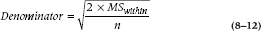
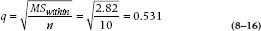
Common to all the remaining methods is the use of the overall Mean Square (Within) as an estimate of the error term in the statistical test, so we’ll elaborate a bit on this idea. You remember in the previous chapter that we spent quite a bit of time devising ways to use the estimate of σ derived from each of the two groups to give us a best guess of the overall SE of the difference. In ANOVA, most of this work is already done for us, in that the Mean Square (Within) is calculated from the differences between individual values and the group mean across all the groups. Furthermore, as we showed already, the Mean Square (Within) is the best estimate of σ2. So the calculation of the denominator starts with Mean Square (Within). We first take the square root to give an estimate of the SD. Finally, we must then divide by some ns to get to the SE of the difference. In the end, the denominator of the test looks like:
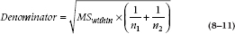
If the sample sizes are the same in both groups, this reduces further to:
For reasons which may, with luck, become evident, we’re going to call this quantity q’. It really represents a critical range of differences between means resulting from the error in the observations. We could, for example, create a t-test using this new denominator:
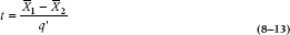
So, in the present example, if we want to compare U to S (the reason for this choice will be obvious in a minute), we would first compute the denominator:
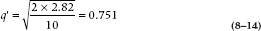
Then, we could proceed with a t-test:
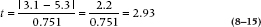
This is just an ordinary t-test, except that we computed the denominator differently, using the Mean Square (Within) instead of a sum of variances, which we called q’. This does introduce one small wrinkle. Since we are using all the data (in this case, 40 observations) to compute the error, we modify the degrees of freedom to take this into account; so, we compare this with a critical value for the t-test on 36 df, which turns out to be 2.03.
In fact, almost all the post-hoc procedures we will discuss are, at their core, variants on a t-test. However, since by definition they involve multiple comparisons (between Group A and Group B, Group A and Group C, etc.), they go about it another way altogether, turning the whole equation on its head, and computing the difference required to obtain a significant result. That is, they begin with a range computed from the Mean Square (Within), multiply it by the appropriate critical value of the particular test, and then conclude that any difference between group means which is larger than this range is statistically significant. Sticking with our example of a t-test for the moment, we would compute the range by multiplying 0.751 by the critical value of the t-test (in this case, 2.03). Then, any difference we encounter that is larger than this, we’ll call statistically significant by the t-test.
Regrettably, before we launch into the litany of post-hoc tests, one more historical diversion is necessary. It seems that, when folks were devising these post-hoc tests, someone decided early on that the factor of 2 in the square root was just unnecessary baggage, so they created a new range, called the Studentized range. This has the formula:
And that’s where q and q’ come about. Why they bothered to create a new range, one will never know. After all, it doesn’t take a rocket scientist to determine that q’ is just  times q. Since most of the range tests use q, we have included critical values of q in Table M in the Appendix.
Fisher’s Least Significant Difference (LSD)
Fisher’s LSD, which is a multiple comparison test, is on the opposite wing in terms of conservatism, and it is actually nothing more than a computational device to save work; goodness knows how this got into the history books. You begin with the critical value of t, given the df. In this case, we have 36 df, so a significant t (at .05) is 2.03. We worked out before that the denominator of the calculated t-test is .751, so any difference between means greater than .751 × 2.03 = 1.52 would be significant. Sooo—1.52 becomes the LSD, and it is not necessary to calculate a new t for every comparison. Just compare the difference to 1.52; if it’s bigger, it’s significant. The formula for the LSD is therefore:
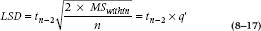
where df is the degrees of freedom association with the MSWithin term. The T – U comparison is still statistically significant. For completeness, the LSD also found the comparison S – U to be significant.
One would be forgiven if there were some inner doubt surfacing about the wisdom of such strategies. Fisher’s LSD does nothing to deal with the problem of multiplicity because the critical value is set at .05 for each comparison; all it does is save a little calculation. But, since computers do the work in any case, that’s not a consideration, and we should avoid using LSD for anything except recreational activities.
Tukey’s Honestly Significant Difference
Perhaps because Tukey saw that LSD did not immortalize Fisher’s name,12 he went the other way and gambled on moral rectitude, coming up with the Honestly Significant Difference (HSD).13
This time the test statistic is changed to something closer to the square root of an F statistic. It has its own table at the back of some stats books (but not this one). In the present example, with 4 and 36 df, the statistic q equals 3.79. Tukey then creates another critical difference, called the Honestly Significant Difference, or HSD:
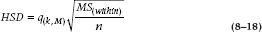
when n is, as before, the sample size in each group, k is the number of groups (4 in this case), and M is the df for the within term, equal to k(n – 1). This time around, then, the HSD equals:
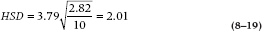
and now the T – U comparison is not significant, but the S – U one still is.
Note that this test, like the one that follows, uses the q statistic. Second, these tests (including the LSD), don’t start with a difference between means and then compute a test statistic, but, rather, start with a test statistic, and compute from it how big the difference between means has to be in order for it to be significant. This involves looking up the critical value of the q statistic in Table M, which turns out to involve not just the mean, SD, and sample size, but also the number of means, k.
This isn’t at all unreasonable. After all, the more groups there are, the more possible differences between group means there are, and the greater the chance that some of them will be extreme enough to ring the .05 bell. So, the test statistic for the HSD and the next test, which we’ve called q up until now, takes all this into account.
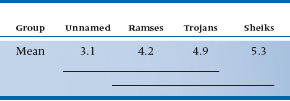
Unlike the previous tests, which were either multiple comparisons (Bonferroni, Holm, Hochberg, and LSD) or range tests (the Studentized Range), the HSD is both. After identifying means that are significantly different, it gives a table showing subsets of homogeneous means, as in Table 8–3. This is interpreted as showing that the means of U, R, and T don’t differ from one another, nor do the means of R, T, and S. A neat way of displaying this is in Table 8–4. The means are listed in numerical order (it doesn’t matter if they’re ascending or descending), and a line is placed under the means that don’t differ from each other. You can use this technique with any range-type post-hoc test.
TABLE 8–3 Tukey’s HSD range test for the data in Table 8–1
| Group | Subset 1 | Subset 2 |
| Unnamed | 3.1 | |
| Ramses | 4.2 | 4.2 |
| Trojans | 4.9 | 4.9 |
| Sheiks | 5.3 |
TABLE 8–4 Displaying the results of Table 8–3 in a Journala
aNote: Means joined by a line are not significantly different.
The Neuman-Keuls Test
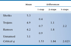
For reasons known only to real statisticians,14 the Neuman–Keuls test appears to have won the post-hoc popularity contest lately. It, too, is a minor variation on what is becoming a familiar theme. We begin by ordering all the group means from highest to lowest.
Now in order to apply the N-K test,15 we have to introduce a new concept, called the step. Basically, we need to know how many steps (means) we have to traverse to get from one mean of interest to the other mean of interest, and what the difference is between the means; we’ve worked this out in Table 8–5. So, to get from S to U, we have four steps; to go from R to U, only one. For α = .05, four means, and 36 degrees of freedom, the tabled value equals 3.81, so any difference between means greater than a critical value of:
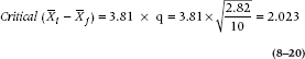
Since the S – U comparison is bigger than 2.023, it is declared significant. Now, to discuss two two-step comparisons. From the table, the critical q is 3.464, so any difference larger than 3.464 × 0.531 = 1.84 is significant. So, T – U is almost, but not quite significant, and S – T is not significant. Since neither comparison is significant, there is no point in continuing, as none of the one-step comparisons would be significant. Just to prove the point, for the one-step comparisons, the critical q is 2.875, so any comparison greater than 2.875 × 0.531 = 1.53 is significant; and none is.
TABLE 8–5 Differences between means for different steps, with critical values of q
Tukey’s Wholly Significant Difference
Tukey’s HSD is the way to go if you have a large number of groups (say, six or more) and you want to make all possible comparisons. The downside is that it tends to be somewhat conservative with respect to Type I and Type II errors. On the other hand, the N-K can be a bit too liberal. Tukey’s Wholly Significant Difference (WSD, also known as Tukey’s b) tries to be like Momma Bear, and be “just right.” If you have k groups, use WSD if you want to do more than k – 1 but fewer than k × (k − 1)/2 comparisons; otherwise, use the N-K.
Dunnett’s t
Yet another t-test. We include it for two reasons only. The big one is that it is the right test for a particular circumstance that is common to many clinical studies in which you wish to compare several treatments with a control group; and second, because Dunnett is an emeritus professor in our department, and the only person named in this book whom we’ve actually met.16
To illustrate the point, returning yet again to the lurid example that got this chapter rolling, one clear difference emerges between R, S, T, and the last one. U you can get for free almost anywhere—student health services, counselors, etc.; whereas, to get R, S, or T, you might have to shell out some hard-earned scholarship dough. Surely, the primary question must be whether the ones you pay for are really any better than the freebies.17 That is, the study is now designed to compare multiple treatments with a control group.18
Dunnett’s test is the essence of simplicity, doing essentially what all the others did. We compute a critical value for the difference using a test statistic called, as you might expect, Dunnett’s t, and another standard error derived from Mean Square (Within), only this time with the  back in—that is, a q’ range. So the critical value looks like:
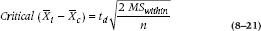
Dunnett’s main contribution was that he worked out what the distribution of the t statistic would be (for reasons of space, you won’t find it in the back of this book). Not surprisingly, like the Studentized range, it is dependent on the number of groups and the sample size. For the present situation, with four groups and a total sample size of 40 (so that df = 40 − 4 = 36), the td is 2.54.19 So, with a Mean Square (Within) of 2.82 the critical value is:
On this basis, brand S, with a difference of 2.2, exceeds this critical value and is declared significantly different from brand U; brands R and T don’t make the grade, regrettably.
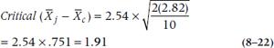
Scheffé’s Method
The last procedure we’ll discuss is also the oldest. Scheffé’s method is intended to be very versatile, allowing any type of comparison you want (for example, A versus B, A versus C, A + B versus C, and so on). To conduct the procedure, you calculate a range, using the overall F-test, the Mean Square (Within), and a complicated little bit of coefficients. It looks like:
For a simple contrast, it’s not quite as bad as it looks. For example, in our present data set, the critical value of F at .05 for 3 and 36 degrees of freedom is 2.88. The number of groups, k, is 4. Mean Square (Within) is, as usual, 2.82. Now taking a simple contrast, if we just wanted to look at the difference between R and U, then C1 is +1, C2 is 0, C3 is 0, and C4 is –1. Putting it all together, the equation is:
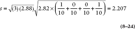
So, any comparison of means greater than 2.207 would be significant at the .05 level. This value is a bit larger than any of the other methods, which is the price you pay for versatility. In fact, Scheffé recommended using the tabled value for α = .10, rather than .05, just to compensate for this conservativeness.
On balance, comparing these methods, it is evident that the LSD method is liberal—it is too likely to find a difference. The Scheffé method is too conservative. One reason for its conservativeness is that it was meant to test all possible comparisons, including highly weird ones. Even if we don’t do all of these comparisons, Scheffé “protects” α from them. In general, the HSD and the Neuman-Keuls methods are somewhere in the middle, although the Neuman-Keuls test is a little less conservative (so we are told). It would seem that most folks these days are opting for the Neuman-Keuls test when they are doing pairwise comparisons. Although we haven’t discussed it, the REGWQ seems to be more powerful than the Newman-Keuls and able to maintain better control over the α level. Dunnett’s test is in a class by itself and should be the method of choice when comparing multiple means to a control mean.
The post-hoc tests we’ve mentioned are all used when we can assume homogeneity of variance among the groups. Because the one-way ANOVA is fairly robust to violations of this assumption, that means they’re used in most situations. If you’re ever faced with severe heterogeneity, then there are four post-hoc tests you can use: Tamahane’s T2, Games-Howell, Dunnett’s T3, and Dunnett’s C.20 Tamahane’s procedure tends to be too conservative, and the Games-Howell too liberal. That leaves us with Dunnett’s two tests, and we don’t find much difference between them.
This pretty well sums up the most popular post-hoc procedures. We have not, by any means, exhausted the space. There are about 25 parametric post-hoc tests, in addition to a multitude of non-parametric and multivariate ones. If you have the fortitude to pursue this further, we have listed a couple of readable references at the back of the book.
PLANNED ORTHOGONAL COMPARISONS
In contrast to these bootstrap methods, planned contrasts are done with a certain élan. The basic strategy is to divide up the signal, the Sum of Squares (Between), among the various hypotheses or contrasts. The sum of squares associated with each is used as a numerator, and the Mean Square (Within) as a denominator, to calculate F-ratios for each test.
To accomplish this sleight of stat, it is necessary to devise the comparisons in a very particular way. If we just went ahead, as we do with post-hoc comparisons, taking differences among means as our whims dictate, then the Sum of Squares associated with all the contrasts would likely add up to more than the Sum of Squares (Between). The reason is that the comparisons overlap—(Mean1 – Mean2), (Mean2 – Mean3), and (Mean3 – Mean1) are, to some degree, capitalizing on the same sources of variance.
To avoid this state of affairs, the comparisons of interest must be constructed in a specific way so that they are nonoverlapping, or orthogonal.
Two things (contrasts, factors, or whatever) are said to be orthogonal if they do not share any common variance.
We ensure that this condition is met by first standardizing the way in which the comparison is written. We do this by introducing weights on each mean. So, each contrast among means is written like:

For example, those condom connoisseurs among the readers probably know that certain, expensive classes can be found among condoms; spermicide present or absent, lubricated or not, and other more architectural differences, the details of which will be spared the reader. Suppose Brands R and S have one such characteristic, and T and U do not. To see if it matters, we would make a comparison as shown:

FIGURE 8-1 Parceling out the Total Sum of Squares into three linear contrasts.
In a similar manner we might like to compare Brand R with Brand S, ignoring T and U. This looks like:

And finally, making the same comparison within the other category ends up looking like:

Now comes the magic. How do we know that these are orthogonal? By multiplying the coefficients together, according to the equation:

where i refers to one contrast and j to the other.
How, you might ask, does this guarantee things are orthogonal? We asked the same question and decided that it was anything but self-evident. Try this, however. Suppose there are two dimensions, X and Y. If we imagine two lines, (a1X + b1X) and (a2X + b2X), they are at right angles (orthogonal) if the sum of the product of the weights is equal to zero.
TABLE 8–6 The ANOVA summary table for the orthogonal comparisons
In this case, the product of the first two sets equals (½)(1) + (½) (−1) + (−½) (0) + (−½) (0) = 0. So far, so good.
Similarly, we have to prove that contrasts 2 and 3 are orthogonal. The sum of weights is (1)(0) + (−1)(0) + (0)(1) + (0)(−1) = 0. We’re getting tired of all this, so you can check the 1 and 3 contrast.
Now that we have established a set of contrasts equal to the number of df, it’s almost easy. We calculate the sum of squares for each contrast as follows:21
- First, calculate the actual contrast. From our data set, they look like:
C1 = ½ × 4.2 + ½ × 5.3 − ½ × 3.1 − ½ × 4.9 = 0.75
C2 = 1 × 4.2 − 1 × 5.3 + 0 × 3.1 + 0 × 4.9 = 1.10
C3 = 0 × 4.2 + 0 × 5.3 + 1 × 3.1 − 1 × 4.9 = −1.80
- Next, calculate the sum of
 , and call it W:
W1 = (½2 + ½2 + ½2 + ½2) ÷ 10 = 1 ÷ 10 = .10
W2 = (12 + 12) ÷ 10 = 2 ÷ 10 = .20
W3 = (12 + 12) ÷ 10 = 2 ÷ 10 = .20
- The sum of squares for each contrast is then, by some further chicanery, equal to C2 ÷ W:
SS(C1) = .752 ÷ .10 = 5.625
SS(C2) = 1.12 ÷ .20 = 6.05
SS(C3) = 1.82 ÷ .20 = 16.2
Stay updated, free articles. Join our Telegram channel

Full access? Get Clinical Tree


