Chapter 4
Mixed models for categorical data
Categorical data often occur in clinical trials. For example, adverse events may be classified on an ordinal scale as mild, moderate or severe. In this chapter we will primarily consider the analysis of measurements made on ordered categorical scales; however, we also describe how unordered categorical data can be analysed. A fixed effects method for analysing ordinal data known as ‘ordinal logistic regression’ was first suggested by McCullagh (1980) and has been widely applied. The mixed categorical model is far less well established. The model that is defined is based on extending ordinal logistic regression to include random effects and covariance patterns. As we suggested in Chapter 3 for GLMMs, some readers with a less statistical background may wish to read only the introductory paragraphs of each section which will enable them to identify where these methods might prove useful. The final section of this chapter and sections of subsequent chapters will illustrate the application of mixed categorical models.
Ordinal logistic regression will be described in Section 4.1. It is extended to a mixed ordinal logistic regression model in Section 4.2. In Section 4.3 we describe how the model can be adapted to analyse unordered categorical data. In Section 4.4 some practical issues related to model fitting and interpretation are considered, and a worked example is given in Section 4.5.
4.1 Ordinal logistic regression (fixed effects model)
Ordinal logistic regression is a fixed effects method for analysing ordinal data. It is often preferable to contingency table methods such as the Chi-squared ‘test for trend’ because several fixed effects can be included in the model. The method works by:
- Assuming observations have a multinomial distribution which can be expressed:

where
- i = observation number,
- j = category number,
- c = number of categories,
 = 1 if
- = 0 otherwise,
- μij = p(yi = j).
- i = observation number,
- Taking the ordered nature of the data into account by defining a model for the cumulative categorical probabilities. The cumulative probabilities,
 , correspond to the probability that observation i is in a category less than or equal to j. They can be thought of as probabilities arising from partitioning the categories in every possible place. For example, if the response variable had categories labelled 1, 2, 3 and 4, three partitions would be possible: 1/2–4, 1–2/3–4 and 1–3/4. The cumulative probabilities are linked to the model parameters using the logit link function (see Section 3.1.4):

where
- Ij = intercept parameter for each partition j,
 =
= 
- xi = ith row of fixed effects design matrix X,
- α = vector of fixed effects parameters.
Note that there is a separate equation for each partition, j.
- Ij = intercept parameter for each partition j,
- Maximising the likelihood function for the model parameters (the Ij and α) based on the multinomial distribution. Methods for maximising the likelihood function coincide with those for the mixed ordinal logistic regression model and are described in Section 4.2. They are based on using the matrix notation below to represent the multinomial distribution.
Expressing the model in matrix notation
The ordinal logistic model can alternatively be expressed using matrix notation. However, the multinomial distribution is not a member of the exponential family and cannot be linked to the model parameters using a single link function. This hurdle can be overcome by re-expressing the data in binary form. To do this we allow each observation to become a vector of c − 1 correlated binary observations (c = number of categories). For example, if there are four categories, then we could let: y = 1 become (1, 0, 0), y = 2 become (0, 1, 0), y = 3 become (0, 0, 1) and y = 4 become (0, 0, 0). Thus, the three terms correspond to the presence or absence of the first three categories, while the presence of the fourth category is implied by the absence of the first three. The vector, y, containing the n extended observations can then be defined as

To illustrate this redefinition consider the following data constituting the first five observations from a repeated measures trial in which y has range 1–4.
| Patient | Visit | Treatment | y |
| 1 | 1 | A | 2 |
| 1 | 2 | A | 1 |
| 1 | 3 | A | 4 |
| 2 | 1 | B | 3 |
| 2 | 2 | B | 1 |
When y is expressed in its extended binary form it becomes

The ordinal logistic model can now be specified in a form of a GLMM using the cumulative probabilities that result from partitioning the categories in each possible place. The GLMM uses a covariance pattern to allow for the multinomial correlations occurring between the binary observations. A cumulative probability,  , is defined as the probability that observation i is in a category less than or equal to j:

μ is the vector of expected multinomial probabilities corresponding to the n extended observations. If there are four categories then we may write

where

μ[c] is a vector containing the cumulative probabilities obtained by partitioning the four categories in the three possible places:

where

So we may equivalently write

α is again a vector containing the fixed effects. It has the same form as given in Section 2.1 except c − 1 intercept terms are included corresponding to each of the c − 1 partitions of the data. Thus, if a model fitting two treatments and three visits as fixed were fitted to the earlier example data, we could write

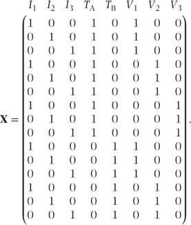
X is again a design matrix for the fixed effects. However, it now has more rows than previously to correspond to the extended number of observations. For our data X would be

Residual matrix
The residual variance matrix, R, needs to take into account the multinomial correlations that occur within the binary vectors used for each observation. From the multinomial distribution it is known that covariances for the observation vectors, (yi1, yi2, …, yi,c − 1)′, are

(E(yijyik) = 0 when j ≠ k because either yij or yik has to be zero.)
Thus, within-observation covariance matrices, Ri, can be defined for each of the n original observations. If c = 4 we can write the covariance terms corresponding to each pair of partitions for observation i as

The Ri matrices form blocks along the diagonal of the full residual matrix, R. For example, in this fixed effects model R is

where

As in the GLMM definition (Section 3.2), R can be arranged as a product of a correlation matrix, P, and the matrix of expected Bernoulli variances, B = diag{μij(1 − μij)}:

Note that the A matrix of constants used for the GLMM is now not required, since the data are in Bernoulli form and A = I. For our example data P may be written as

where

4.2 Mixed ordinal logistic regression
The fixed effects ordinal logistic model can be easily extended to a mixed ordinal logistic regression model by adding random effects terms and allowing covariance patterns in the residual matrix.
In Section 4.2.1 the ordinal mixed model will be specified. The residual matrix for mixed categorical models has a more complex form than for GLMMs and will be defined in Section 4.2.2. As in GLMMs, there can be benefits in reparameterising random effects models as covariance pattern models and this will be discussed in Section 4.2.3. A quasi-likelihood function for the model is defined in Section 4.2.4, and model fitting methods are discussed in Section 4.2.5.
4.2.1 Definition of the mixed ordinal logistic regression model
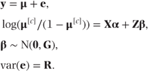
The ordinal mixed model can now be specified as

β is a vector containing the random effects. Thus, if a model fitting two treatments and three visits as fixed and patients as random were fitted to the earlier example data, we could write

Z is the design matrix for the random effects and has additional rows than previously to correspond to the extended number of observations. For our data, Z would be

The  matrix
G is again a matrix of variance parameters corresponding to the random effects and coefficients and has the same form as given in Section 2.1. In the model we have considered, fitting one random effect (patient) G would have the form

where
 = patient variance component.
4.2.2 Residual variance matrix
The residual variance matrix, R, needs to take into account, first, the multinomial correlations that occur within the binary vectors used for each observation (see Section 4.1) and, second, any covariance patterns defined at the residual level. As in Section 4.1, we arrange R as B1/2PB1/2, a product of a correlation matrix, P, and the matrix of expected Bernoulli variances, B.
In a covariance pattern model the correlation matrix, P, will include off-diagonal blocks of correlation parameters. For example, if a general covariance pattern was used to model our example data, then we would require a separate block of correlations for each pair of time points and P would have the form

Note that the diagonal matrix blocks will differ for each observation as indicated at the end of Section 4.1. The Pmn are (c − 1) × (c − 1) = 3 × 3 submatrices of parameters corresponding to the correlation between observations at visits m and n on the same patient. They replace the single correlation values used in GLMMs, and here we assume they take the form

with a separate correlation parameter used for each pair of partitions. Thus, six parameters are used for each Pmn matrix here. This is the parameterisation used by Lipsitz et al. (1994) who has written an accompanying SAS macro for fitting the model in this form. However, because this model requires more covariance parameters than GLMMs, particularly when the number of categories is high (increased by a factor of c(c − 1) / 2), more complex covariance patterns should be used with caution.
Simpler parameterisation for covariance pattern models
Here, we suggest an alternative simpler parameterisation with just one parameter corresponding to each of the parameters in the original covariance pattern (i.e. one for compound symmetry, three here for a general pattern). The correlation matrix for our example using a general covariance pattern would be

Stay updated, free articles. Join our Telegram channel

Full access? Get Clinical Tree


