Finally, the model does not separate drug-specific (efficacy and affinity) and tissue-specific (receptor density) parameters. The drug-specific pharmacodynamic parameters have been found to be remarkably consistent among different species and from in vitro studies (1). Thus, if an integrated PK–PD model for drug response in vivo separated the drug- and tissue-specific parameters, it would be possible to estimate drug response in humans based on parameters found in laboratory animals or in vitro. This translational research could have a major impact on drug development. It could allow drug candidates with the greatest chance of success to be identified early during development and could help to optimize the design of clinical trials, which could decrease both the cost and time of drug development. The sigmoidal E_max parameters are, however, dependent on both the drug and the system in which they were determined. As a result, this model has limited applications in translational research.

The disadvantages of the sigmoidal E_max model have been addressed through the development of a range of mechanism-based pharmacodynamic models that incorporate additional steps in the chain of events between receptor activation and the emergence of the response [see (1–3)]. A description of some of these models is presented below.

17.2 MODELS INCORPORATING RECEPTOR THEORY: OPERATIONAL MODEL OF AGONISM

As discussed above, the parameters of the sigmoidal E_max model are combined drug- and tissue-specific parameters. Black and Leff’s operational model of agonism (4) incorporates receptor theory into in vivo models of drug response. As a result, the model provides estimates of the drug-specific parameters of efficacy and affinity.

As presented in Chapter 16, according to classical receptor theory, the interaction of a drug with its receptors is controlled by the law of mass action. The concentration of receptors occupied is expressed as follows:

(17.1)

where RC is the concentration of the drug–receptor complex, C the concentration of drug, R_T the total concentration of receptors, and K_d the drug’s dissociation constant, a reciprocal measure of a drug’s affinity. Furthermore, the response that results from the drug–receptor interaction is believed to be a function of the number of receptors occupied:

(17.2)

where E is the effect and E_m is the maximum possible response of the system.

The E_max model is mathematically equivalent to the intrinsic activity model, which assumes a linear relationship between response and receptor occupancy (Figure 17.2). As shown previously [equations (16.15) and (16.16)], E_max is equivalent to the product of the maximum response of the system or the maximum response of a full agonist, and the intrinsic activity: E_max = E_m · α (Note: For full agonists, α = 1; for partial agonists, 0 < α < 1). As a result, E_max is both a drug-specific (α) and a system-specific (E_m) parameter. This model also assumes that full agonists will all produce the same quality of drug–receptor interaction and that a given fractional occupancy will produce the same response among different drugs. But this is not necessarily the case, as many drugs are able to produce a maximum response at less than 100% receptor occupancy.

FIGURE 17.2 Relationship between fractional receptor occupancy and response for the E_max model (upper panel) and the operation model of agonism (lower panel). K_d is an inverse measure of affinity and corresponds to the drug concentration that results in 50% receptor occupancy. The E_max model is equivalent to a model that assumes that the response (E) is directly proportional to the fraction of receptors occupied (RC/R_T). The OMA assumes a hyperbolic relationship between response and receptor occupancy. K_e or RC_E50 is the drug–receptor concentration that results in 50% of the system’s maximum response.

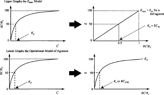
The Black and Leff operational model of agonism (4) is an alternative way of modeling drug action. The model accommodates the concept of spare receptors and incorporates a term to represent a drug’s efficacy, which enables it to distinguish among full agonists that have different efficacies. Thus, it addresses the fact that the response to a given level of receptor occupancy varies among drugs, and that a maximum response can be observed at less than 100% receptor occupancy.

The normal hyperbolic, capacity-limited relationship between drug concentration and receptor occupancy is assumed [equation (17.1)]. A second hyperbolic capacity-limited process is then used to model the relationship between the concentration of the drug–receptor complex and the response (Figure 17.2):

(17.3)

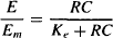
where E_m is the maximum possible response of the system (as distinct from E_max, which is the maximum possible response of a given drug) and K_e is the concentration of the drug–receptor complex that produces 50% E_m.

This model allows the response elicited by a given drug–receptor concentration to vary among drugs. Drugs with higher efficacy will be able to elicit a given effect at a lower drug–receptor concentration than will drugs with low efficacy. The K_e value (Figure 17.2, lower right) is the concentration of the drug–receptor complex that produces half the maximum response of the system. A more meaningful symbol for K_e is RC_E50. Thus, RC_E50 is a measure of efficacy. Drugs with low RC_E50 values will be able to produce 50% of the system’s maximal response at lower drug–receptor complex concentrations than will drugs with high RC_E50 values.

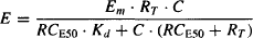
Substituting the expression for RC shown in equation (17.1) into equation (17.3), we have

(17.4)

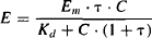
Equation (17.4) is simplified by introducing an efficacy expression known as the transduction ratio (τ), which is defined as the ratio of the total concentration of receptors to the concentration of drug–receptor complex that produces 50% of the maximum response (R_T/RC_E50). The larger the value of the transduction ratio, the greater is a drug’s efficacy. If, for example, a relatively low concentration of the drug–receptor complex produces a 50% maximum response (RC_E50 is small), the transduction ratio (τ) is large.

Substituting for the transduction ratio in equation (17.4), the response may be expressed as

(17.5)

The parameters of the E_max model (E_max and EC₅₀) can be related to those of the operational model of agonism (OMA). When a drug’s response is maximum (E = E_max), C is high, C >> K_d, and the expression in the denominator of equation (17.5) may be modified: K_d + C + C · τ = C + C · τ:

(17.6)

A drug’s EC₅₀ is the concentration that produces half of the drug’s maximum response. Substituting for E_max/2 for E and EC₅₀ for C in equation (17.5) yields

(17.7)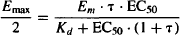

Substituting for E_max from equation (17.6), and rearranging, we have

(17.8)

Full agonists with high intrinsic efficacy can produce a large response at relatively low concentrations (Figure 16.3). They will have low RC_E50 values and, as a result, high transduction ratios. The denominator in equation (17.6) will then simplify to 1 + τ ≈ τ, and the drug’s E_max will be the system maximum. For example, if τ = 99, EC₅₀ = K_d/100, and E_max = (99% E_m). The fact that the EC₅₀ is much less than the K_d (the drug concentration when 50% of the receptors are occupied) illustrates that the drug has high efficacy. This drug, which is able to produce the full system response, can produce half the maximum response when only about 1% (1/99 × 100%) of the receptors are occupied. If a drug has a low τ (e.g., 0.01), EC₅₀ is approximately equal to K_d and the maximum effect is about 1% of E_m (4). When τ = 1, the agonist produces half of the system’s maximum response at 100% receptor occupancy, and this constitutes the drug’s E_max [E_max = E_m · τ/(1 + τ) = E_m/2]. This would occur with a partial agonist or in a tissue that either had a low concentration of receptors or one in which the receptors had become desensitized.

This model can also incorporate a slope factor (n) similar to the slope factor of the sigmoidal E_max model. The model equations that incorporate this factor are

(17.9)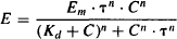

(17.10)

(17.11)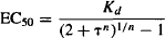

In clinical studies, the values of E_m and n can be determined using a full agonist and the sigmoidal E_max model. The response–concentration data can then be modeled to determine τ and K_d. The OMA has been used extensively in studies on the μ-opioid (MOP) agonists. It was used to successfully simulate the effects of a series of MOP agonists in rats using values of the affinity and efficacy determined in vitro, in conjunction with system-specific parameters (E_m and n), (5). Determination of the transduction ratio in vivo has enabled the relative efficacies of some MOP agonists to be determined in mice [see (6)]. These studies found an efficacy of fentanyl > etorphine > methadone = morphine > hydromorphone > oxycodone > hydrocodone. In another study conducted in rats, the development of tolerance to alfentanil was associated with large increases in the drug’s EC₅₀. Theoretically, this could be explained by either a decrease in affinity or a decrease in efficacy. Simulations performed using the OMA demonstrated that the observations could be explained by a 40% loss of functional MOP receptors (7), which indicated that normally the system has a very large receptor reserve (5,7).Since drug-specific parameters have been found to be consistent between species, the OMA is expected to be of great value in translational research where studies conducted in vitro or in animal models generate drug-specific parameters, which can then be applied to humans (1,8).

17.2.1 Simulation Exercise

Open the model “Operational Model of Agonism” at the link

http://www.uri.edu/pharmacy/faculty/rosenbaum/basicmodels.html#chapter17a

The model has the following default parameters: RC_E50 = 5 mg/L, R_T = 200 units, K_d = 10 mg/L, and E_m = 100%. A problem based on the OMA (Problem 17.1) reviews the properties and behavior of the model.

17.3 PHYSIOLOGICAL TURNOVER MODEL AND ITS CHARACTERISTICS

The direct action of a drug can be modeled using the sigmoidal E_max model, any of its derived models (E_max and linear models), or the operational model of agonism. Mechanism-based PK–PD models address the events that occur along the response chain subsequent to the receptor activation and the generation of the initial stimulus (Figure 17.1). For example, models have been developed to address long transduction processes, the development of tolerance, indirect drug effects, irreversible drug effects, and the impact of drugs on an underlying disease that changes over time (disease progression models). A variety of different models have been developed to address these issues, and many incorporate a physiological turnover model for the synthesis and degradation of a biological quantity or factor (Figure 17.3). These turnover models were first introduced into pharmacodynamics with the indirect effect models (9–12) and have subsequently been incorporated into other models in diverse and creative ways. In pharmacodynamic models, the biological factor (R) that is being produced in the turnover model is an entity that is usually directly involved in mediating the biological response. As a result, it is often referred to as the response variable. In models, R has been a variety of different things, including the amount or concentration of an endogenous compound, an enzyme, white blood cells, red blood cells, and gastric acid secretion. Most commonly, formation of the biological quantity is assumed to be a zero-order process with a rate constant of k_in. Loss or degradation of R is assumed to be a first-order process with a rate constant of k_out.

FIGURE 17.3 Turnover model for the formation and loss of a biological factor or response variable (R). Its formation is assumed to be a zero-order process (k_in), and loss is assumed to be first order with a rate constant of k_out.

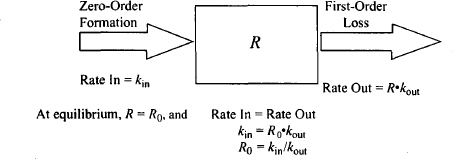
The physiological system for the production and degradation of the biological factor is shown in Figure 17.3. The assumptions and characteristics of the system are as follows:

• It is assumed that the precursor pool for the biological factor is very large and is never depleted. As a result, it is assumed to be formed by a constant continuous (zero-order) process: rate = k_in.
  
• The factor is assumed to be degraded or removed by a first-order process, the rate of which is dependent on the value of the factor and a first-order rate constant k_out.
  
• The rate of change of R with time is given by
  
  

  (17.12)

  where R is a biological quantity, k_in is a zero-order rate constant for the formation of R, and k_out is a first-order rate constant for the loss of R.
  
• Under normal circumstances, the system is stationary and at equilibrium. The biological factor (R) will be constant and have a baseline level of R₀. At baseline,

rate of production = rate of degradation

(17.13)

Rearranging yields

(17.14)

17.3.1 Points of Drug Action

External factors such as drugs and/or disease can interfere with the physiological system through actions on k_in and/or k_out, or by a direct effect on R. These actions would destroy the equilibrium and produce changes in R. An inhibition of k_in, a stimulation of k_out, or direct destruction of the biological factor would all result in a decrease its value. In contrast, stimulation of k_in or inhibition of k_out would increase the value of the biological factor.

17.3.2 System Recovery After Change in Baseline Value

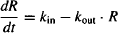
Assuming that the action of the external influence is only temporary, once the influence is removed, the system would return to equilibrium and its normal baseline level. Figure 17.4 shows how the values of k_in and k_out influence the return to baseline after an external influence reduced the response variable to 50% of its normal baseline value. It can be seen that the time for the system to restore equilibrium is dependent on k_out and independent of k_in. Since the loss of the biological factor is a first-order process, it takes about 4 degradation (k_out) half-lives for equilibrium to be restored (Appendix B). The system is analogous to the kinetics of an intravenous infusion, where the time to steady state is dependent on a drug’s elimination half-life and independent of the infusion rate and the value of the steady-state plasma concentration. In common with the infusion model, the time it takes for the system to restore equilibrium is also independent of the magnitude of the initial change. Thus, if the baseline is disrupted by 20, 50, or 70%, it will still take 4 degradation (k_out) half-lives for equilibrium to be restored.

FIGURE 17.4 Influence of the values of the rate constants on the time it takes a system to restore equilibrium when the baseline is reduced by 50%. Values of k_out of 0.05, 0.1, and 0.2 h⁻¹ were used, and k_in was set to 10 units/h. Values of k_in of 5, 10, and 20 units/h were used and k_out was fixed at 0.1 h⁻¹. Response is fractional change from baseline.

In summary:

• The time it takes the system to restore the usual baseline level is dependent on the value of k_out. As a first-order process, it will take 3 to 5 k_out half-lives for the system to return to baseline.
  
• The time it takes the system to restore the usual baseline level is independent of the value of k_in.
  
• The time it takes the system to restore the usual baseline level is independent of the magnitude of the change from baseline.

17.4 INDIRECT EFFECT MODELS

The product of a physiological system such as the one discussed above may be a natural ligand (R) that is directly responsible for a physiological response. For example, R could be gastric acid production, a substance that clots blood, or a low-density lipoprotein. A drug could exert its action by affecting the concentration of R. It could reduce R either by inhibiting its formation or by stimulating its degradation. Alternatively, it could increase R by either stimulating its production or inhibiting its degradation. Such drugs are said to act indirectly. Warfarin is an example of a drug that acts indirectly. Warfarin is used therapeutically to inhibit the clotting of blood, but it does not have any direct effect on this process. Instead, it inhibits the synthesis of clotting factors that play an integral part in the clotting of blood, and it is the concentration of these clotting factors (response variables) that is directly related to the action of warfarin.

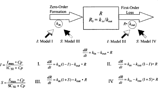
Pharmacodynamic models for drugs that act indirectly need to incorporate, in addition to the model for the drug’s direct action (e.g., E_max model), the physiological turnover system described above. The four potential ways that drugs can interfere with the physiological turnover models [inhibition or stimulation of either k_in or k_out (Figure 17.5)] give rise to four basic indirect models (9):

FIGURE 17.5 Four indirect effect models. Drugs could inhibit k_in or k_out (models I and II, respectively) or stimulate k_in or k_out (models III and IV, respectively).

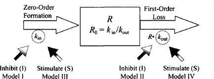
• Inhibition of k_in: model I
  
• Inhibition of k_out: model II
  
• Stimulation of k_in: model III
  
• Stimulation of k_out: model IV
  
  

The direct action of a drug on the physiological system is usually modeled using the E_max or sigmoidal E_max model. To differentiate the four models, the “effect” is categorized as either stimulation (S) or inhibition (I), and it is measured as the fractional change in the rate constant affected. Thus, the stimulatory (S) or inhibitory (I) effect of 03 would mean a 30% increase or a 30% decrease, respectively, in the rate constant affected. The equations for the direct effect of the drug are

(17.15)

(17.16)

where I and S represent the fractional change in the rate constant, I_max is the maximal possible fraction inhibition that a drug can produce [(I_max can vary between zero (no inhibition) and 1 (complete inhibition)], IC₅₀ the drug concentration that produces 50% of I_max. S_max the maximal fraction stimulation that a drug can produce (S_max can be any number greater than zero), and SC₅₀ the drug concentration that produces 50% of S_max. Cp is the plasma concentration, which is assumed to drive the direct effect.

The action of the drug on k_in or k_out is then incorporated into the differential equation for the physiological model [equation (17.12)]. For example, for model I, the inhibition of k_in the inhibitory action of the drug, would be incorporated as follows:

(17.17)

Substituting I from equation (17.15) into equation (17.17), we have

(17.18)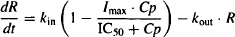

The equations for all four indirect effect models are shown in Figure 17.6. It is not possible to solve the differential equations to obtain explicit solutions. As a result, simulations are extremely useful in understanding the characteristics of indirect effect models.

FIGURE 17.6 Equations for the four indirect models. The rate of change of the response variable (R) with time is equal to the rate in minus the rate out. The direct effect of the drug to either inhibit (I) or stimulate (S) k_in or k_out is modeled using the E_max model. The direct effect is expressed in terms of the fraction decrease (inhibition) or increase (stimulation) in the rate constant affected.

17.4.1 Characteristics of Indirect Effect Drug Responses

Indirect effect models have been used extensively to model the response of a variety of drugs, including the action of warfarin on the synthesis of clotting factors; the inhibitory action of H2-blockers on acid secretion; the inhibition of water reabsorption by furosimide, bronchodilation produced by β₂-agonists, and the action of terbutaline in reducing potassium concentrations (13).

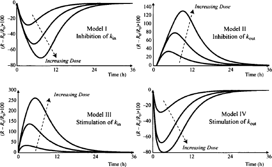
In two of the four models the drug reduces the response variable (inhibition of k_in and stimulation of k_out), while in the other two models the drug increases the response variable above its baseline (stimulation of k_in and inhibition of k_out). Figure 17.7 shows the typical response profiles from the four indirect effect models at three dose levels. The data were simulated by connecting a one-compartment model with intravenous bolus input to each of the four indirect effect models. Two special characteristics of these models are clearly visible in Figure 17.7. First, the response is delayed relative to the plasma concentration (with an intravenous injection, the peak plasma concentration occurs at time zero). Second, although, as expected, the maximum response (R_m) increases with dose, unusually, the time of the maximum response (T_Rm) also increases with dose.

FIGURE 17.7 Response (percent change from baseline) profiles of the four indirect effect models after a series of intravenous bolus injections. Simulations were performed using doses of 10, 100, and 1000 mg in each of the four models. The models had the following parameters: Vd = 20 L, k = 0.7 h⁻¹, k_in = 10 units/h, k_out = 0.2 h⁻¹, I_max (models 1 and II) = 1, S_max (models III and IV) = 5, IC₅₀ (models I and II) = 0.1 mg/L, SC₅₀ (models III and IV) = 1 mg/L.

The four models share many characteristics and some have their own unique features. A detailed discussion of the properties of the models, the selection of an appropriate model for a specific drug effect, and the estimation of model parameters are beyond the scope of this discussion but can be found in the literature (10–12). The discussion below will provide a general description of the models, with particular emphasis on how the model parameters affect the time course of drug response (the onset, magnitude, and duration) and how this affects the design of dosing regimens. The discussion is presented using model I, the inhibition of k_in, as the example. Interactive simulation models of all four indirect models are provided to allow readers to evaluate the characteristics of all the indirect effect models.

17.4.2 Characteristics of Indirect Effect Models Illustrated Using Model I

In the indirect effect model I, the drug inhibits the zero-order rate constant (k_in) for the production of the response variable. This model has been applied to the action of warfarin, which is used widely to increase the clotting time of blood in patients who are susceptible to blood clots and at risk for strokes. Warfarin exerts its action by inhibiting the synthesis of clotting factors that are involved in the clotting process. Indirect effect model I results in a decrease in the value of the response variable according to the equation

(17.19)

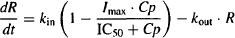
If high concentrations of the drug are able to inhibit k_in completely, I_max = 1 and the parameter can be removed from the numerator. Initially, when no drug is present, the response is at its equilibrium baseline value (k_in/k_out) (see Figure 17.3). After an intravenous dose, assuming no distributional delays, the drug will immediately inhibit k_in, and the synthesis of the response variable will fall. Translation of the drug action into a decrease in the response variable itself will depend on the time it takes for the existing response variable to be removed, which will depend on the value of k_out.

The characteristics of the model will be demonstrated using simulations. A one-compartment model with intravenous bolus input was combined with the indirect effect model. The simulations were carried out using the following default parameter values: dose = 100 mg, k = 0.7 h⁻¹, Vd = 20 L, IC₅₀ = 0.1 mg/L, I_max = 1, k_in = 10 units/h, and k_out = 0.2 h⁻¹. Note that for these simulations, k > k_out; the loss of the response variable is rate limiting (the drug’s elimination half-life is shorter than the half-life for the turnover of the response variable). The model used to simulate these figures may be found at

http://www.uri.edu/pharmacy/faculty/rosenbaum/basicmodels.html#chapter17b

17.4.2.1 Time Course of Response

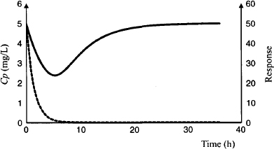
Note that for clarity the elimination half-life of the drug has been set to 1 h. The time course of the response can be observed in Figure 17.8; the plasma concentration (dashed line) is at its peak at time zero, but the maximum response does not occur until about 5 h (5 elimination half-lives). At this time, the drug has been almost completely removed from the body. For drugs with indirect action, the time course of the drug action extends beyond the drug’s presence in the body. In this example, it takes about 16 h (16 drug elimination half-lives) for the baseline to return to about 90% of its original value. Recall from Section 17.3.2 that once the external force is removed, it takes about 4 k_out half-lives for the system to be restored to equilibrium. In this example the t_1/2 of k_out is 3.5 h.

FIGURE 17.8 Plasma concentration (dashed line) and response (solid line) after an intravenous bolus injection (100 mg). Simulations were carried out using parameter values for model I given in the legend of Figure 17.7.

17.4.2.2 Effect of Dose

It was shown previously (Figure 17.7) that as the value of the dose increases, the response increases. Note, however, that the dose–response relationship is nonlinear. In model I, a dose of 10 produces a maximum response (R_m) of about a 25% change from baseline, a dose of 100 produces an R_m of about a 50% change from baseline, and a dose of 1000 mg produces an R_m of about a 70% change from baseline. Also note that the time for the maximum response (T_RM) increases with dose. This is characteristic of these models and can be used to distinguish delays in response caused by indirect effects from delays caused by a slow distribution of the drug to its site of action. Recall that in the effect compartment model, the time for the maximum response remains constant with dose (see 16.5.1). The time of the maximum effect in the indirect models increases with dose because larger doses produce greater saturation of the system (e.g., receptors) and, as a result, the duration of the direct action of the drug is longer (see Figure 16.12b). Because k_in is inhibited for a longer period at higher doses, the peak or maximum response occurs later. Thus, the duration of action of action increases with dose.

17.4.2.3 Maximum Response and Maximum Achievable Response of a Drug

At the peak response (R_m), the rate of production of the response variable equals the rate of removal, and the rate of change of R with time is momentarily zero:

(17.20)

Substituting into (17.19) and rearranging gives us

(17.21)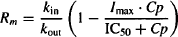

Substituting for k_in/k_out according to equation (17.14) yields

(17.22)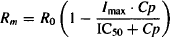

As the dose increases the drug’s effect (I) approaches I_max and R_m approaches the maximum effect the drug can achieve (R_max), since Cp >> IC₅₀, IC₅₀ + Cp ≈ Cp and:

(17.23)

If a drug has the maximum possible value of I_max (1), R_max tends to zero and the response expressed as the percentage change from baseline tends to 100%. Thus, the maximum response possible in model I is zero.

17.4.2.4 Influence of Physiological System Parameters

When the physiological turnover system was studied in isolation earlier in the chapter, it was shown that the time for complete recovery of the system after its equilibrium has been disturbed, is dependent on k_out and independent of k_in. The independence of recovery on k_in for the indirect effect model is shown in Figure 17.9a, which shows the time course of the therapeutic response (expressed as a percentage change from baseline) at three values of k_in. The influence of k_out on the system is shown in Figure 17.9b. Note that k_out controls both the onset of action and the recovery of the system. The larger the value of k_out, the faster the onset, the shorter T_Rm and the faster the recovery. This has important implications for dosing regimen design. Small values of k_out will result in a long duration of action and will enable the drug to be administered less frequently. When the k_out is 0.05 h⁻¹ (k_out t_1/2 = 14 h), the action of the drug persists for over 36 h. Thus, this drug could easily be administered daily, even though it has an elimination half-life of 1 h.

FIGURE 17.9 Effect of variability in the three rate constants on a response profile in indirect effect model 1 after IV bolus administration. Response is the percent change from baseline. In part (a), k_in was varied (5, 10, and 20 units/h); in part (b), k_out was varied (0.05, 0.1, and 0.3 h⁻¹), with k at its default value (0.7 h⁻¹); in part (c), k_out was varied (0.2, 0.4, and 0.8 h⁻¹) with k set to 0.1 h⁻¹); and in part (d), k was varied (0.35, 0.7. and 1.4 h⁻¹). The dose was set to 100 mg. Unless otherwise stated, all other parameters were set to the default values given in the legend of Figure 17.7.

Figure 17.9c shows the influence of k_out in a system where k_out > k (elimination is rate controlling). Note that the time scale of this plot has been expanded to 72 h. Under these circumstances (k < k_out), k_out has little influence on the duration of action. Elimination is a rate-limiting process and it controls the duration of action. The dosing interval of the drug would then be based on the pharmacokinetic not the pharmacodynamic characteristics of the drug.

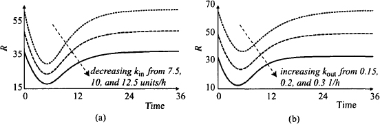
The initial values of k_in and k_out determine the baseline value of the biological variable. As a result, when the initial value of either parameter is altered, the baseline and the absolute change in R will be affected (Figure 17.10). It can be seen that smaller values of k_in are associated with lower baseline values of R. The response curve is shifted downward and the maximum response is greater, but recall from Figure 17.9a that the relative change in R is the same for all values of k_in. It can be seen that as the initial value of k_out increases, the baseline decreases and the response curve is shifted downward. A given dose produces a larger maximum response, which occurs earlier (recall from Figure 17.9b that larger initial values of k_out also produce larger relative responses). The smaller the value of k_out, the longer it takes to return to baseline.

FIGURE 17.10 Effect of changes in k_in and k_out on the absolute value of the response variable (R). The values of the rate constants that were varied are given in the figure. All other parameter values were set to their default values given in the legend of Figure 17.7.

17.4.2.5 Influence of Pharmacokinetics: Elimination Rate Constant

The elimination rate constant is a measure of the rate of drug elimination. It can be seen (Figure 17.9d) that slower elimination (smaller values of the elimination rate constant) results in increased maximum responses, an increase in T_Rm, and a more prolonged duration of action of the drug. Slower elimination results in a more prolonged inhibition of k_in, which will result in a more profound, longer-lasting therapeutic effect. The value of k does not affect the onset of response (the initial slope).

17.4.2.6 Pharmacodynamic Parameters of the Drug: Effect of IC₅₀ and I_max

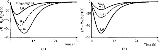
Variability in IC₅₀ is essentially the same as variability in the dose. A decrease in the value of IC₅₀ (the potency of the drug increases) is equivalent to an increase in the dose. Thus, when IC₅₀ decreases, the response and the time for maximum response increase (Figure 17.11a). In contrast, as the I_max value increases, the response increases but the time for maximum response remains the same (Figure 17.11b). Note that variability in I_max produces proportional changes in R_m.

FIGURE 17.11 Effect of variability in IC₅₀ (a) and I_max (b) on the response profile of indirect effect model I after IV bolus administration. Response (percent change from baseline) was simulated using values of IC₅₀ of 0.01, 0.1, and 1 mg/L (a) and values of I_max of 0.25, 0.5, and 1 (b). A dose of 100 mg was used, and unless otherwise stated, all other parameters were set to the default values given in the legend of Figure 17.7.

17.4.2.7 Time to Steady State During an Intravenous Infusion

The time to steady-state response during a constant, continuous intravenous infusion is shown in Figure 17.12. Figure 17.12a shows the response over time for model I and, for comparison, Figure 17.12b shows the response for model IV (stimulation of k_out), which also produces a reduction in the response variable below baseline. Note that for model I (Figure 17.12a) the time to steady-state response is about the same for the various infusion rates, and it is approximately 24 h. In contrast, the time to steady-state response in model IV decreases as the infusion rate increases (Figure 17.12b). This is because the value of k_out controls the time to steady-state response. In model I, k_out does not vary with dose; it is constant (0.2 h⁻¹, k_out t_1/2 = 3.5 h), and by about 7 k_out half-lives (24.5 h), the response is at steady state. In contrast, k_out is the subject of the drug’s action in model IV. Larger infusion rates will produce larger stimulations of k_out, and as a result (k_out

Stay updated, free articles. Join our Telegram channel

Join