Epidemiology is a quantitative discipline. It involves the collection of data within a study sample and analyses using statistical methods to summarise, examine associations and test specific hypotheses from which it infers generalisable conclusions about aetiology (causes of disease) and health care evaluation in the target population. In order to be able to understand epidemiological research, one must have a basic understanding of the statistical tools that are used for data analysis both in epidemiological and basic science research.

Types of variables

A variable is a quantity that varies; for example, between people, occasions or different parts of the body. A variable can take any one of a specified set of values. Medical data may include the following types of variables.

Numerical variables

There are two types of numerical variables. Continuous variables are measurements made on a continuous scale; for example, height, haemoglobin or systolic blood pressure. Discrete variables are counts, such as the number of children in a family, or the number of asthma attacks in a week.

Categorical variables

There are two basic types of categorical variable, which are variables that take nonnumeric values and refer to categories of data. Firstly, unordered categorical variables are used to class observations into a number of named groups; for example, ethnic group, marital status (single, married, widowed, other), or disease categories. A special case of the unordered categorical variable is one which classes observations into two groups. Such variables are known as dichotomous or binary and generally indicate the presence or absence of a particular characteristic. Presence versus absence of chest pain, smoker versus nonsmoker, and vaccinated versus unvaccinated are examples of dichotomous or binary variables.

Secondly, ordered categorical variables are used to rank observations according to an ordered classification, such as social class, severity of disease (mild, moderate, severe), or stages in the development of a cancer. Often in epidemiological studies a variable may be measured as numerical and then subsequently categorised. For example height may be measured in feet and inches and then categorised as: <5ft, 5ft–5ft 5in, 5ft 5in–6ft, >6ft.

The type of variable will determine how that variable is displayed and what subsequent analyses are carried out. In general, continuous and discrete variables are treated in the same way.

Descriptive statistics for numerical variables

Most medical, biological, social, physical and natural phenomena display variability. Frequency distributions express this variability and are summarised by measures of central tendency (‘location’) and of variability (‘spread’). We will explore these measures using the following hypothetical data on the number of days spent in hospital by 19 patients following admission with a diagnosis of an acute exacerbation of chronic obstructive airways disease.

Measures of central tendency

There are three important measures of central tendency or location.

1. Mean

The mean is the most commonly used ‘average’. It is the sum of all the values in a set of observations divided by the number of observations in that set.

So the mean number of days spent in hospital by the 19 patients is

The algebraic formula for this calculation is given in Table 2.1.

2. Median

The median is the middle value when the values in a set are arranged in order. If there is an even number of values the median is defined as the mean of the two middle values.

Thus, the median number of days spent in hospital is 10 days (see Figure 2.1).

3. Mode

The mode is the most frequently occurring value in a set. It is rarely used in epidemiological practice.

The modal number of days spent in hospital is 8 days.

For data presented in grouped form, e.g. if hospital stay were grouped as 0–10, 11–20, 21–30 and 30+ days, we can identify the modal class in this instance as 0–10 days. Thought of in this way, it is a peak on a frequency distribution or histogram. When there is a single mode, the distribution is known as unimodal. If there is more than one peak the distribution is said to be bimodal (two peaks) or multimodal.

Figure 2.1 Distribution of hospital stay in sample of 19 patients.

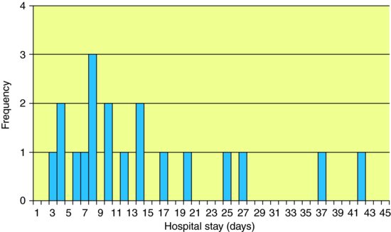
Table 2.1 Formulae for the mean and standard deviation.

Let us assume in the above example that the patient with the longest length of stay actually spent 120 days rather than 42 days in hospital because they could not be sent back home but required placement in a nursing home. This ‘unusual’ observation (outlier) would have a large effect on the mean value (now 18.6 days) whilst having no effect on the median and could make the performance of one hospital look worse than another depending on which summary statistic was being used for the comparison.

Measures of variability

The extent to which the values of a variable in a distribution are spread out a long way or a short way from the centre indicates their variability or spread. There are several useful measures of variability.

1. Range

The range is simply the difference between the largest and the smallest values.

The range of the number of days spent in hospital following operation for the 19 patients is:

As a measure of variability, the range suffers from the fact that it depends solely on the two extreme values which may give a quite unrepresentative view of the spread of the whole set of values.

2. Interquartile range

Quantiles are divisions of a set of values into equal, ordered subgroups. The median, as defined above, delimits the lower and upper halves of the data. Tertiles divide the data into three equal groups, quartiles into four, quintiles into five, deciles into ten, and centiles into 100 subgroups. Measures of variability may thus be the interquartile range (from the first to the third quartile), the 2.5th to 97.5th centile range (containing the ‘central’ 95% of observations, and so on).

For example, the quartiles for the data on days spent in hospital are 7, 10 and 20 days, so the interquartile range is: 7 days to 20 days

3. Standard deviation

The standard deviation (SD) is a measure of spread of the observations about the mean. It is based on the deviations (differences) of each observation from the mean value: these deviations are squared to remove the effect of their sign. The SD is then calculated as the square root of the sum of these squared deviations divided by the number of observations minus 1.

The SD of the data on days spent in hospital is calculated as:

The algebraic formula for this calculation is given in Table 2.1. The square of the SD (that is, SD × SD) is known as the variance.

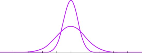
The Normal (or Gaussian) distribution (introduced in Chapter 1) is described entirely by its mean and standard deviation (SD). The mean, median and mode of the distribution are identical and define the location of the curve. The SD determines the shape of the curve, which is tall and narrow for small SDs and short and wide for large ones (see Figure 2.2).

Figure 2.2 Normal distribution curves. The flatter, wider curve has a greater standard deviation.

Stay updated, free articles. Join our Telegram channel

Join