Fig. 17.1
Four parameter logistic regression with asymptotes A and D, 50th percentile C and slope B
A model derived from Michaelis-Menten kinetics is the four-parameter logistic regression equation:
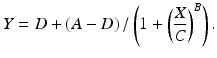
In this version of the model the parameters A and D represent the upper and lower asymptotes, respectively, C is the concentration corresponding to half the range in the asymptotes, (A − D)/2, and B is a slope parameter. The parameter C is sometimes denoted EC50 for the half maximal effective concentration or IC50 for the half maximal inhibitory concentration, and is used as a measure of the absolute potency of a test material in some laboratories. A five parameter logistic model incorporates a parameter for asymmetry of the concentration response curve, and is discussed in Gottschalk (2005).
(17.1)
USP General Chapter <1032> on Design and Development of Biological Assays recommends the use of a reference standard to report the relative potency of a test material to the standard. In this design the reference standard is assayed alongside the test material to reduce the variability due to influences of the biological system on assay responses. The design of such a bioassay is called a parallel curve design (Fig. 17.2).
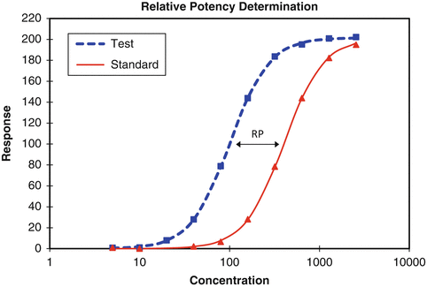
Fig 17.2
Parallel curve design yielding a relative potency (RP) of test to standard
In the model associated with this design the test material is assumed to behave as a dilution (shifted right, requiring higher concentrations to achieve the same response profile as the standard) or as a concentration (shifted left, requiring lower concentrations) of the reference standard. It is further assumed that the shift is constant across the range of responses in the assay. This condition of a constant shift is called similarity or parallelism between the test and reference curves. A test of similarity is performed prior to the calculation of relative potency (see Sect. 17.2.4).
As discussed in Sect. 17.2.1, the number of concentrations and concentration increment should account for the projected range of potencies and the mathematical model which will be utilized to translate the responses to the measure of potency. When the four parameter logistic model is used, sufficient numbers of concentrations should be planned to assess similarity (two points across the range of potencies on the asymptotes) and to obtain a robust estimate of relative potency (four points across the range of potencies in the approximately linear region of the curve). The combined requirements usually result in selection of 10–12 concentrations to span the range to be tested. Some laboratories adjust the concentration series to satisfy the assumptions when the test material is expected to vary significantly from the standard (for example, forced degradation samples).
A special case of nonlinear modeling is applied to quantal responses (number of positives). Analyses can be performed after a linearizing transformation of the responses (probit or logit transformation). Similar considerations are used for the design of quantal response bioassay as parallel curve bioassay. The models used to assess similarity and to fit the data will be discussed in Sect. 17.2.3.
17.2.2.2 Linear Models
Among the linear models used to fit bioassay data are parallel line and slope ratio models. Both models use a reference standard to calculate the relative potency of the test material to the standard. One may be considered over the other based on the distribution of responses at each concentration. The parallel line model is more appropriate if the distribution of responses (for example, instrument readout) is approximately log-normal, and characterized by proportional increase in the variability (standard deviation) of the responses with increase in the level of response. The slope ratio model might be used if the distribution is approximately normal and the variability is constant across levels.
A design consideration associated with these two models is the concentration scaling. For reasons of the regression characteristics of either model (that is, symmetric weighting across concentrations), geometric scaling should be used to create the series for the parallel-line model while arithmetic scaling should be used in conjunction with the slope ratio model. The conditions required to support a slope ratio model are infrequently met in current bioassays. Further details on the analysis of slope ratio bioassays are given in USP General Chapter <1032> Design and Development of Biological Assays and <1034> Analysis of Biological Assays.
Linear models are derived from the nonlinear model in one of two ways. One is based on selection of concentrations in the “linear” region of the full concentration response curve (Fig. 17.3).
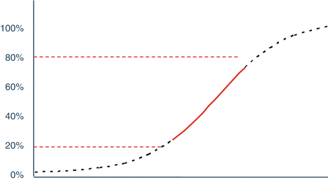
Fig 17.3
Approximately linear region of concentration response curve (20–80 %)
The linear region is typically selected to contain concentrations yielding 10–90 % or 20–80 % of maximal response, and should include at least three or four concentrations to satisfy the requirements for the assessment of curvature and parallelism as well as the determination of relative potency. This is managed through the selection of the concentration scaling in correspondence to the steepness of the linear portion of the concentration response curve, as well as consideration of the expected potencies to be tested. As with parallel curve design the laboratory may vary the concentration series of a test material which is expected to significantly vary from the reference standard (for example, forced degradation samples).
A second linear model derives from the lower region of the full concentration response curve (Fig. 17.4).
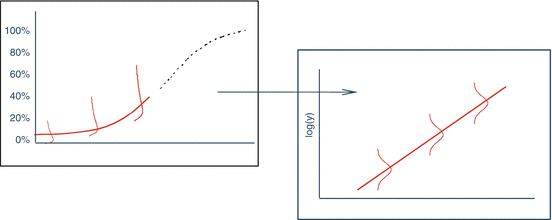
Fig 17.4
Log transformation of the lower region of curve linearizes the curve and normalizes the residuals
This lower region can be linearized using a log-log fit to the data. This approach has optimal properties as will be discussed in Sect. 17.2.2.3.
17.2.2.3 Selection of a Model
The selection of a model depends upon a number of considerations including technical constraints, efficiency, variability of the biological system and regulatory requirements. Technical constraints include such things as the numbers of wells across a row or a column of a plate or availability of data processing software. Efficiency is a consideration for bioassays used for high throughput screening or to support large process development studies. The variability of the biological system should be considered in conjunction with the ability to effectively manage the concentration series across the range of samples which will be tested in the bioassay. Regulatory authorities may differ in their preference towards one model over another.
Technical, efficiency and regulatory considerations notwithstanding, nonlinear models may be preferred over their linear counterparts. This is because the nonlinear models relate better to the kinetics principles underlying bioassay concentration response than their linear approximations. Between the linear approximations selection of the lower portion of the concentration response profile has practical as well as statistical advantages. One of these advantages stems from the distributions of most bioassay responses. Responses such as luminescence are typically log-normally distributed. Thus a log-log fit to the curve both linearizes the curve and transforms response into an appropriate scale for analysis. Another advantage stems from the variability of the biological system and the range of potencies. When the biological system or potency range varies the linear region shifts towards one or another of the asymptotic regions of the curve. These shifts induce parallelism failures which can result in biased estimates of potency for a test material (see Sect. 17.2.5).
The absolute potency of the reference standard may be used as a system suitability test rather than (or in addition) to calculate relative potency. This may be appropriate when the biological system is tightly controlled, and determination of relative potency may increase variability due to compounding the variability of the standard together with the variability of the test material. Use of the reference standard for relative potency determination or as a system suitability test can be assessed utilizing correlation analysis on paired measurements [ where i indexes the test (T) and standard (S)] in the bioassay. The paired measurements might be made as duplicate series of the reference standard as part of the determination of an acceptance criterion for similarity (see Sect. 17.2.4). Using a formula for the log of the relative potency (see Sect. 17.2.6),
  , the variance of M is given by:
The variability of relative potency determination may exceed that of C T when:
![$$ Var\left({C}_T^{'}\right)>2\cdot Cov\left({C}_S^{‘},{C}_T^{‘}\right). $$
” src=”/wp-content/uploads/2016/07/A330233_1_En_17_Chapter_Equ3.gif”></DIV></DIV><br />
<DIV class=EquationNumber>(17.3)</DIV></DIV>In this case the laboratory might prefer to report <SPAN class=EmphasisTypeItalic>C</SPAN> <SUB><SPAN class=EmphasisTypeItalic>T</SPAN> </SUB>rather than relative potency. Care should be taken, however, to consider the lifecycle of the bioassay. Absolute potency is susceptible to differences in conditions and reagents between laboratories. Relative potency should be used if the method will be transferred to other laboratories.</DIV></DIV><br />
<DIV></DIV><br />
<DIV id=Sec8 class=]()
Get Clinical Tree app for offline access

where i indexes the test (T) and standard (S)] in the bioassay. The paired measurements might be made as duplicate series of the reference standard as part of the determination of an acceptance criterion for similarity (see Sect. 17.2.4). Using a formula for the log of the relative potency (see Sect. 17.2.6), , the variance of M is given by:(17.2)
17.2.3 Model Fitting
Nonlinear or linear regression models are used to fit bioassay responses, assess similarity and determine potency. Standard statistical approaches to fitting and assessing these models will be discussed. These include consideration of the scale of responses, assessment of outliers and goodness-of-fit of the statistical model.
17.2.3.1 Scale of Responses
As in typical regression the assumptions of the method should be evaluated prior to fitting a model. Key assumptions are that the residuals from the regression are approximately normally distributed and the variability of responses is homogeneous across levels. Many bioassays yield non-normal responses owing to the bound of 0 on response measurement and the inherent nature of the biological response. In many bioassays the scale of the responses is approximately log-normal. Inattention to the scale of responses can lead to instability of procedures for assessing similarity and outliers as well as increases in variability of potency measurement.
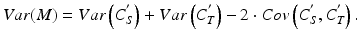
As the conditions of non-normality of responses and heterogeneity of variability are related, these can be assessed through simple statistical tools such as residual plots or through replication studies. The residual plot (Fig. 17.5) from a curve or series of curves exhibiting log-normal (heterogeneous variability) behavior is characterized by increasing spread in residuals with increasing level of response (or concentration for increasing concentration response bioassays).
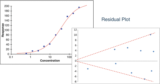
Fig 17.5
Residual plot showing increasing variability with increasing concentration
A study with independent replicates at each concentration may also reveal heterogeneous variability (Fig. 17.6).
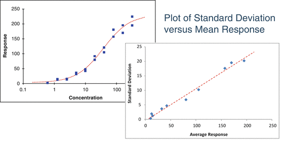
Fig 17.6
Plot of standard deviation versus average response
Several approaches can be utilized to mitigate the impact of heterogeneity of variability on potency determination. Two of these are to perform weighted regression or to transform the responses. A weighted regression is performed by minimizing the weighted sum of squares for error.
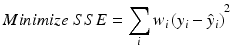
where
 Alternatively a transformation can be performed using a Box-Cox transformation of the responses (the residuals).
The log-likelihood of the power function can be used to read off the power λ and 95 % confidence interval. If the confidence interval includes 0 this is evidence towards log transformation.
(17.4)
(17.5)
Transformation may be preferred to weighted regression because transformation usually generates responses which meet conditions both of normality and homogeneity of variability. Transformation also reduces the apparent excess variability in responses in the region of the upper asymptote of the fitted model. That variability may cause excess false positive assessments of similarity and can mask important properties in the data such as a “hook” or prozone effect. In principle the transformed data are unlikely to follow Michaelis-Menten kinetics; however, this departure from the theoretical kinetics is typically outweighed by the improved statistical properties of the transformed data. Probit and logit analysis of quantal response bioassay data are performed using recursive weighted regression.
17.2.3.2 Outlier Analysis
Outlier analysis is sometimes performed on replicates to detect individual responses which may be due to mechanical error (missed well, pipetting error, etc.) or some other special cause variation. Approaches include replication based and model based outlier methods.
Replication based outlier methods look at groupings of replicates to determine one or more potential outliers. It is important to assess scale of response prior to outlier analysis. In particular log-normally distributed responses may appear to contain outliers due to the skewed nature in the distribution of responses. Most commonly employed methods such as Grubb’s test or Dixon’s test described in USP Chapter <111> Design and Analysis of Biological Assays, assume normality of the underlying distribution. Other methods such as range charting and residual analysis use an estimate of the response variability to assess when a range among replicates or a residual is beyond usual performance in the bioassay. These methods should be restricted to replicates which are independent and not linked to replicates in other groupings. Pseudo-replicates derived from aliquots of a common sample concentration may be assessed as a group. True replicates derived from independent dilutions series should not be assessed as a group. This is because the special cause variation may derive from the series rather than the individual replicate. Finally replication based outlier methods are typically insensitive due to the small number of replicates.
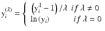
Model based outlier methods utilize the residuals from the fits of an appropriate bioassay model to the concentration response data (Fig. 17.7). As these depend upon an appropriate model, goodness-of-fit of the model should be performed prior to outlier analysis (see Sect. 17.2.3.3).
Fig 17.7
Example of a model residual
Simple methods such as dividing the residual by an estimate of the root mean square error after removal of the suspect outlier are available in some software packages, while graphical methods such as residual plots or probability plots may serve this purpose. While methods for calculating standardized residuals (that is, residuals divided by their standard error) are documented for linear models, these are more difficult to calculate for nonlinear models. Additional considerations for the assessment of outliers include:
For parallel curve or parallel line bioassay the residuals should be obtained from the unconstrained (individual parameter) fits to the curves.
Care should be taken to assess an outlier against the appropriate estimate of variability (for example, pseudo replicates should be assessed using a different estimate of variability than replicates derived from different series).
The actions taken when one or more outliers are detected vary. Some laboratories will exclude the individual outliers while others may exclude a dilution or dilutions associated with the outliers. The lab should assess the impact of exclusion of the outlier on similarity testing and relative potency determination. If removal of the outlier shifts the decision regarding similarity or compliance with the potency specification, care should be taken to err on the side of the conservative decision. In spite of the availability of outlier tools a lab may choose to forego the practice of outlier analysis after performing an assessment of the impact of outliers on the determination of similarity and potency in a bioassay.
17.2.3.3 Goodness-of-Fit
Goodness-of-fit (GOF) of the bioassay model constitutes a test or set of tests to establish that the model used to fit the responses provides an acceptable description of the data. For linear models statistical measures such as R-squared are used to assess GOF. It can be shown, however, that curvilinear data can yield a satisfactory R-squared (see Anscombe 1973; Chatterjee and Firat 2007). The European Pharmacopeia (EP) Chapter 5.3 describes a test of curvature to establish that a linear model provides an acceptable fit to the data. That test suffers, however, from addressing the wrong hypothesis. The conclusion from the test is that there is insufficient evidence to conclude curvature, which is not the same as concluding that there is acceptable linearity. An amended version of the EP test might be to establish a metric of curvature (for example, the quadratic coefficient) and a margin of acceptability for the metric. This is analogous to the approach which is described for similarity or parallelism (see Sect. 17.2.4).
Additional heuristic approaches can be applied to both linear and nonlinear models. A plot of the residuals will reveal patterns which may be expected to occur when the model generates a poor fit to the data (for example, quadratic curvature for the linear model or runs of positive and negative residuals for a nonlinear model). Finally the lab may address lack of fit during development by assuring the fit with a higher order model such as a quadratic or nonlinear model.
17.2.4 Test of Similarity
A test of similarity (also called test of parallelism in the case of a linear model) is used in the processing of bioassay data to warrant that the kinetics of a test material is similar to that of a standard (except for a shift along the concentration scale). This is a requirement in parallel line and parallel curve bioassay (Fig. 17.8), but should also be assessed against the control when an absolute measure of potency (for example, EC50) is reported. The test is used both biologically to establish that the kinetics of the test material has not changed due to an alteration in its primary or secondary structure, and/or operationally to warrant the measurement of relative potency.
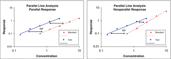
Fig 17.8
Parallel and nonparallel concentration responses between test and standard materials
A test of similarity was traditionally performed as part of the analysis of variance (see EP 5.3) using an F-test statistic that is constructed by comparison of the error sums of squares of the unconstrained model (individual fits to the test and standard data) and constrained model (parameters constrained to be equal for the test and the standard). The curves are determined to be equivalent when the F-test statistic is less than an appropriate percentile of the F-distribution. As previously, the conclusion when the test requirement is satisfied is that there is insufficient evidence to conclude that the curves are dissimilar. This is not the same as concluding that the curves are similar.
An alternative method described in USP <1032> is to test similarity using an equivalence approach. This begins with choosing a metric of similarity. In parallel line bioassay this might be the difference or the ratio of slopes between the linear fits to the test and standard data. The ratio may be preferred as it is unitless and can be formulated as a percent difference relative to the standard slope. A metric of similarity for a slope ratio bioassay is the difference in intercepts from the linear fits.
A metric (or metrics) of similarity for parallel curve bioassay is complicated by the fact that there are multiple parameters which describe the shape of the curve (for example, A, B and D in four parameter logistic regression). Methods for reducing these to one or two metrics follow:
A chi-square test is described in Gottschalk and Dunn (2005). The chi-square test statistic is the numerator of the F-test statistic described in EP 5.3, and is proposed because of the reduced sensitivity to the precision of the unconstrained fit. As described in the article the chi-square test statistic is compared to the appropriate percentile of the chi-square distribution. An alternative is to use the chi-square statistic as a metric for equivalence testing.
Two functions of the model parameters which describe meaningful properties of the biological response are the slope (B) and the range (A-D) of the fitted curve. The difference (or ratio) between the fits to the test and standard data may be used as metrics of similarity between the curves. Because these are likely to be highly correlated, one of these or a multivariate combination should be considered.
In bioassays with increasing response with increasing concentration the lower asymptote (D) estimates the background response of the biological system. Since this is a property of the system and not a property of the test and standard materials the metrics may be reduced to the maximum (A) and the slope (B). Similar consideration should be given to the correlation between A and B as above.
Once a metric (or metrics) has been selected an equivalence margin and rule are established to test similarity. USP <1032> Design and Development of Biological Assays describes four approaches.
1.


The distribution of the metric can be estimated from a sampling of bioassay runs containing a pair of samples. The pair may be duplicates of the reference standard (sometimes referred to as ref-ref pairs) or the reference standard and a control. Statistical process control (SPC) limits can be developed based on the data or on simulations made from properties which affect the similarity metric(s). Since the designation of test and reference is arbitrary, the maximum difference of the percentile from the expected value (zero if the difference, one if the ratio) should be used as the margin. The bounds for the ratio may be set geometrically to account for the behavior of a ratio statistic. A test sample will be judged similar if the calculated value for the metric falls within the equivalence margin.
< div class='tao-gold-member'>
Only gold members can continue reading. Log In or Register to continue
Stay updated, free articles. Join our Telegram channel
Full access? Get Clinical Tree