Exposure and Response after a Single Dose

Kinetics Following an Intravenous Bolus Dose

OBJECTIVES

The reader will be able to:

• Define the meaning of the following terms: clearance, compartmental model, disposition kinetics, distribution phase, elimination half-life, elimination phase, elimination rate constant, extraction ratio, extravasation, first-order process, fraction excreted unchanged, fraction in plasma unbound, fractional rate of elimination, glomerular filtration rate, half-life, hepatic clearance, loglinear decline, mean residence time, monoexponential equation, renal clearance, terminal phase, tissue distribution half-life, volume of distribution.
  
• Estimate from plasma and urine data following an intravenous (i.v.) dose of a drug:
  
  
  
  • Total clearance, half-life, elimination rate constant, and volume of distribution.
    
  • Fraction excreted unchanged and renal clearance.
  
  
• Calculate the concentration of drug in the plasma and the amount of drug in the body with time following an i.v. dose, given values for the pertinent pharmacokinetic parameters.
  
• Ascertain the relative contribution of the renal and hepatic routes to total elimination from their respective clearance values.
  
• Describe the impact of distribution kinetics on the interpretation of plasma concentration–time data following i.v. bolus administration.
  
• Determine the mean residence time of a drug when plasma concentration–time data after a single bolus dose are provided.
  
• Explain the statement, “Half-life and elimination rate constant depend upon clearance and volume of distribution, and not vice versa.”

dministering a drug intravascularly ensures that the entire dose enters the systemic circulation. By rapid injection, elevated concentrations of drug can be promptly achieved; by continuous infusion at a controlled rate, a constant concentration, and often response, can be maintained. With no other route of administration can plasma concentration be as promptly and efficiently controlled. Of the two intravascular routes, the i.v one is the most frequently employed. Intra-arterial administration, which has greater inherent manipulative dangers, is reserved for situations in which drug localization in a specific organ or tissue is desired. It is achieved by inputting drug into the artery directly supplying the target tissue.

The disposition characteristics of a drug are defined by analyzing the temporal changes of drug in plasma and urine following i.v. administration. How this information is obtained following rapid injection of a drug, as well as how the underlying processes control the profile, form the basis of this chapter, Chapter 4, Membranes and Distribution, and Chapter 5, Elimination. These are followed by chapters dealing with the kinetic events following an extravascular dose and the physiologic processes governing drug absorption. The final chapter in this section of the book deals with the time course of drug response after administering a single dose. The concepts laid down in this section provide a foundation for making rational decisions in therapeutics, the subject of subsequent sections.

APPRECIATION OF KINETIC CONCEPTS

Toward the end of Chapter 2, we considered the impact that various shapes of the exposure-time profile following an oral dose may have on the clinical utility of a drug. Figures 3-1 and 3-2 provide a similar set of exposure–time profiles except that the drugs are now given as an i.v. bolus. Notice that following the same dose, the two drugs displayed in Fig. 3-1 have the same initial concentration but different slopes of decline, whereas those displayed in Fig. 3-2 have different initial concentrations but similar slopes of decline. The reasons for these differences are now explored.

Several methods are employed for graphically displaying plasma concentration–time data. One common method that has been mostly employed in the preceding chapters and shown on the left-hand side of Figs. 3-1 and 3-2 is to plot concentration against time on regular (Cartesian) graph paper. Depicted in this way, the plasma concentration is seen to fall in a curvilinear manner. Another method of display is a plot of the same data on semilogarithmic paper (right-hand graphs in Figs. 3-1 and 3-2). The time scale is the same as before, but now, the ordinate (concentration) scale is logarithmic. Notice now that all the profiles decline linearly and, being straight lines, make it easier in many ways to predict the concentration at any time. But why do we get a linear decline when plotting the data on a semilogarithmic scale (commonly referred to as a loglinear decline), and what determines the large differences seen in the profiles for the various drugs?

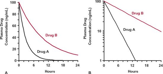
FIGURE 3-1. Drugs A (black line) and B (colored line) show the same initial (peak) exposure but have different half-lives and total exposure–time profiles (AUC). A. Regular (Cartesian) plot. B. Semilogarithmic plot. Doses of both drugs are the same.

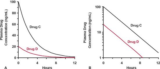
FIGURE 3-2. Drugs C (black line) and D (colored line) have the same half-life but have different initial concentrations and total exposure–time profiles. A. Regular (Cartesian) plot. B. Semilogarithmic plot. Doses of both drugs are the same.

VOLUME OF DISTRIBUTION AND CLEARANCE

To start answering these questions, consider the simple scheme depicted in Fig. 3-3. Here, drug is placed into a well-stirred reservoir, representing the body, whose contents are recycled by a pump through an extractor, which can be thought of as the liver or kidneys, that removes drug. The drug concentrations in the reservoir, C, and that coming out of the extractor, C_out, can be measured. The initial concentration in the reservoir, C(0), depends on the amount introduced, Dose, and the volume of the container, V. Therefore,

Fluid passes through the extractor at a flow rate, Q. With the concentration of drug entering the extractor being the same as that in the reservoir, C, it follows that the rate of presentation to the extractor is then Q · C. Of the drug entering the extractor, a fraction, E, is extracted (by elimination processes) never to return to the reservoir. The corresponding rate of drug leaving the extractor and returning to the reservoir is therefore Q · C_out. The rate of elimination (or rate of extraction) is then:

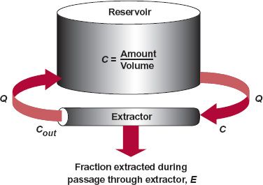
FIGURE 3-3. Schematic diagram of a perfused organ system. Drug is placed into a well-stirred reservoir, volume V, from which fluid perfuses an extractor at flow rate Q. The rate of extraction can be expressed as a fraction E of the rate of presentation, Q · C. The rate that escaping drug returns to the reservoir is Q · C_out. For modeling purposes, the amount of drug in the extractor is negligible compared to the amount of drug contained in the reservoir.

Rate of elimination = Q · C · E = Q(C − C_out)               3-2

from which it follows that the extraction ratio, E, of the drug by the extractor is given by

Thus, we see that the extraction ratio can be determined experimentally by measuring the concentrations entering and leaving the extractor and by normalizing the difference by the entering concentration.

Conceptually, it is useful to relate the rate of elimination to the measured concentration entering the extractor, which is the same as that in the reservoir. This parameter is called clearance, CL. Therefore,

Rate of elimination = CL · C               3-4

Note that the units of clearance are those of flow (e.g., mL/min or L/hr). This follows because rate of elimination is expressed in units of mass per unit time, such as μ-g/min or mg/hr, and concentration is expressed in units of mass per unit volume, such as μg/L or mg/L. An important relationship is also obtained by comparing the equalities in Eqs. 3-2 and 3-4, yielding

CL = Q · E               3-5

This equation provides a physical interpretation of clearance. Namely, clearance is the volume of the fluid presented to the eliminating organ (extractor) that is effectively, completely cleared of drug per unit time. For example, if Q = 1 L/min and E = 0.5, then effectively 0.5 L of the fluid entering the extractor from the reservoir is completely cleared of drug each minute. Also, it is seen that even for a perfect extractor (E = 1) the clearance of drug is limited in its upper value to Q, the flow rate to the extractor. Under these circumstances, we say that the clearance of the drug is sensitive to flow rate, the limiting factor in delivering drug to the extractor.

Two very useful parameters in pharmacokinetics have now been introduced, volume of distribution (volume of the reservoir in this example) and clearance (the parameter relating rate of elimination to the concentration in the systemic circulation [reservoir]). The first parameter predicts the concentration for a given amount in the body (reservoir). The second provides an estimate of the rate of elimination at any concentration.

FIRST-ORDER ELIMINATION

The remaining question is: How quickly does drug decline from the reservoir? This is answered by considering the rate of elimination (CL · C) relative to the amount present in the reservoir (A), a ratio commonly referred to as the fractional rate of elimination, k

or

This important relationship shows that k depends on clearance and the volume of the reservoir, two independent parameters. Note also that the units of k are reciprocal time. For example, if the clearance of the drug is 1 L/hr and the volume of the reservoir is 10 L, then k = 0.1 hr⁻¹ or, expressed as a percentage, 10% per hour. That is, 10% of that in the reservoir is eliminated each hour. When expressing k, it is helpful to choose time units so that the value of k is much less than 1. For example, if instead of hours, we had chosen days as the unit of time, then the value of clearance would be 24 L/day, and therefore k = 2.4 day⁻¹, implying that the fractional rate of elimination is 240% per day, a number which is clearly misleading.

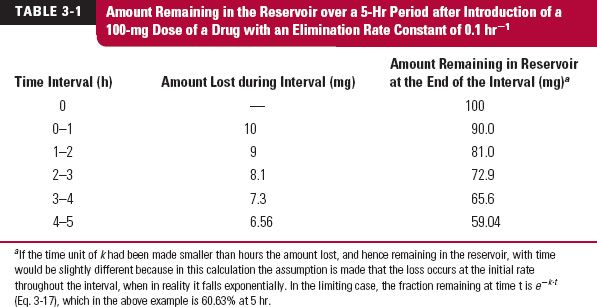
To further appreciate the meaning of k, consider the data in Table 3-1, which shows the loss of drug in the reservoir with time, when k = 0.1 hr⁻¹. Starting with 100 mg, in 1 hr, 10% has been eliminated, so that 90 mg remains. In the next hour, 10% of 90 mg, or 9 mg, is eliminated, leaving 81 mg remaining at 2 hrs, and so on. Although this method illustrates the application of k in determining the time course of drug elimination, and hence drug remaining in the body, it is rather laborious and has some error associated with it. A simpler and more accurate way of calculating these values at any time is used (see “Fraction of Dose Remaining” later in this chapter).

Considering further the rate of elimination, there are two ways of determining it experimentally. One method mentioned previously is to measure the rates entering and leaving the organ. The other method is to determine the rate of loss of drug from the reservoir, since the only reason for the loss from the system is elimination in the extractor. Hence, by reference to Eq. 3-6

where — dA is the small amount of drug lost (hence the negative sign) from the reservoir during a small interval of time dt. Processes, such as those represented by Eq. 3-8, in which the rate of the process is directly proportional to the amount present, are known as first-order processes, in that the rate varies in direct proportion with the amount there raised to the power of one (A¹ = A). For this reason, the parameter k is frequently called the first-order elimination rate constant. Then, substituting A = V · C on both sides of Eq. 3-8, and dividing by V gives

which, on integration, yields

C = C(0) · e^−k·t               3-10

where e is the natural base with a value of 2.71828 . . . Equation 3-10 is known as a mono-exponential equation, in that it involves a single exponential term. Examination of this equation shows that it has the right properties. At time zero, e^−k·t = e⁻⁰ = 1, so that C = C(0) and, as time approaches infinity, e^−k·t approaches zero and so therefore does concentration. Equation 10 describes the curvilinear plots in Figs. 3-1 and 3-2. To see why such curves become linear when concentration is plotted on a logarithmic scale, take the logarithms of both sides of Eq. 3-10.

ln C = ln C(0) — k · t               3-11

where ln is the natural logarithm. Thus, we see from Eq. 3-11 that ln C is a linear function of time with a slope of — k, as indeed observed in Figs. 3-1 and 3-2. Moreover, the slope of the line determines how fast the concentration declines, which in turn is governed by V and CL, independent parameters. The larger the elimination rate constant k the more rapid is drug elimination.

HALF-LIFE

Commonly, the kinetics of drugs is characterized by a half-life (t_1/2), the time for the concentration (and amount in the reservoir) to fall by one half, rather than by an elimination rate constant. These two parameters are of course interrelated. This is seen from Eq. 3-10. In one half-life, C = 0.5 × C(0), therefore

0.5 × C(0) = C(0) · e^−k·t_½               3-12

or

e^−k·t_½ = 0.5               3-13

which, on inverting and taking logarithms on both sides, gives

Further, given that ln 2 = 0.693,

or, on substituting k by CL/V, leads to another important relationship, namely,

From Eq. 3-16, it should be evident that half-life is controlled by V and CL, and not vice versa.

To appreciate the application of Eq. 3-16, consider creatinine, a product of muscle catabolism and used as a measure of renal function. For a typical 70-kg, 60-year-old patient, creatinine has a clearance of 4.5 L/hr (75 mL/min) and is evenly distributed throughout the 42 L of total body water. As expected by calculation using Eq. 3-16, its half-life is 6.5 hr. Inulin, a polysaccharide also used to assess renal function, has the same clearance as creatinine in such a patient, but a half-life of only 2.5 hr. This is a consequence of inulin being restricted to the 16 L of extracellular body water (i.e., its “reservoir” size is smaller than that of creatinine).

FRACTION OF DOSE REMAINING

Another view of the kinetics of drug elimination may be gained by examining how the fraction of the dose remaining in the reservoir (A/Dose) varies with time. By reference to Eq. 3-10 and multiplying both sides by V

Sometimes, it is useful to express time relative to half-life. The benefit in doing so is seen by letting n be the number of half-lives elapsed after a bolus dose (n = t/t_1/2). Then, as k = 0.693/t_1/2, one obtains

Since e^−0.693 = 1/2, it follows that

Thus, one half or 50% of the dose remains after 1 half-life, and one fourth (½ × ½) or 25% remains after 2 half-lives, and so on. Satisfy yourself that by 4 half-lives, only 6.25% of the dose remains to be eliminated. You might also prove to yourself that 10% remains at 3.32 half-lives.

If one uses 99% lost (1% remaining) as a point when the drug is considered to have been for all practical purposes eliminated, then 6.64 half-lives is the time. For a drug with a 9-min half-life, this is close to 60 min, whereas for a drug with a 9-day half-life, the corresponding time is 2 months.

CLEARANCE, AREA, AND VOLUME OF DISTRIBUTION

We are now in a position to fully explain the different curves seen in Figs. 3-1 and 3-2, which were simulated applying the simple scheme in Fig. 3-3. Drugs A and B in Fig. 3-1A have the same initial (peak) concentration following administration of the same dose. Therefore, they must have the same volume of distribution, V, which follows from Eq. 3-1. However, Drug A has a shorter half-life, and hence a larger value of k, from which we conclude that, since k = CL/V, it must have a higher clearance. The lower total exposure (area under the curve [AUC]) seen with Drug A follows from its higher clearance. This is seen from Eq. 3-4, repeated here,

Rate of elimination = CL · C

By rearranging this equation, it can be seen that during a small interval of time dt

Amount eliminated in interval dt = CL · C · dt               3-20

where the product C · dt is the corresponding small area under the concentration–time curve within the time interval dt. For example, if the clearance of a drug is 0.1 L/min and the AUC between 60 and 61 min is 0.1 mg-min/L, then the amount of drug eliminated in that minute is 0.01 mg. The total amount of drug eventually eliminated, which for an i.v. bolus equals the dose administered, is assessed by adding up or integrating the amounts eliminated in each time interval, from time zero to time infinity, and therefore,

Dose = CL · AUC               3-21

or, rearranging,

where AUC is the total exposure. Thus, returning to the drugs depicted in Fig. 3-1, since the clearance of Drug A is higher, its AUC must be lower than that of Drug B for a given dose. Several additional points are worth noting. First, because clearance, calculated using Eq. 3-22

Stay updated, free articles. Join our Telegram channel

Join