Chapter 4
In-Market Product Forecasting
The most essential qualification for a politician is the ability to foretell what will happen tomorrow, next month, and next year, and to explain afterwards why it did not happen.
Winston Churchill
No data yet. It is a capital mistake to theorise before you have all of the evidence.
Sherlock Holmes
The previous chapter explored forecasting methods that are applicable prior to a product’s launch into the market. With the advent of a product’s introduction into the market a new consideration comes into play – the generation of time-series data. This chapter will present techniques related to in-market (also called current product) forecasting. As discussed in Chapter 2, the methods available to the forecaster now include statistical time-series tools in addition to the judgment rich methods discussed in the prior chapters (see Figure 2.7).
Does this mean that the forecaster can use purely statistical techniques to evaluate historical data and project future trends? If so, shouldn’t the forecasts become more ‘accurate’ as the uncertainty inherent in judgmental data disappears? The answer to both questions is ‘absolutely not.’ We will explore the justification for this answer in this chapter, presenting best practices for in-market forecasting.
In-Market Product Forecast Algorithm
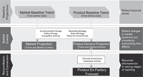
The general algorithm used for in-market forecasting is shown in Figure 4.1. This algorithm can modified for specific therapy areas and products, but the general sections of the algorithm remain invariant: trend historical data, apply the effects of ex-trend events, and convert the trended data into the required forecast outputs.
Figure 4.1 Generalized in-market product forecast algorithm
Trending Historical Data
The first step in the algorithm is to use historical data to examine market and product performance. Trending the historical data is often viewed as a purely statistical exercise, where a software program accepts the historical data inputs and returns a ‘best fit’ trend line that projects performance into the future. In the simplest case, this trending occurs when an individual simply places a ruler against a graph of historical data points and draws a projected line into the future. The subtleties of trending, however, are much more complex, and selecting the appropriate approach for trending historical data is the first key judgment a forecaster makes for in-market forecasting.
TRENDING ALGORITHMS
In Chapter 2 various methods for trending time-series data were presented in Figure 2.7. A definition of each of these statistical techniques is given in Appendix B. There are a number of software programs available to the forecaster; each software package performs these varied trending algorithms almost effortlessly. Every valid approach seeks to fit the time-series data to a trend line that minimizes the deviation between the actual data and the predicted data from the trending algorithm (usually referred to as minimization of the root mean square error of the trend). Differences in software packages arise primarily from the user interfaces (both for input and output of the data) and the number of potential methods used to fit the historical data points. Almost all trending software programs will handle complexities such as seasonality.
Many excellent software reviews have been conducted on trending algorithms.1 Rather than repeat these reviews here we will focus on two key challenges to the forecaster in performing trend analysis: selecting the underlying datasets to trend and selecting the appropriate number of historical data points for the analysis.
SELECTING THE UNDERLYING DATASETS TO TREND
The pharmaceutical industry is both blessed and cursed by data. There are a number of data sources and inputs available for time-series analysis: total prescriptions, new prescriptions, total units, units by stock-keeping unit, units by strength, days of therapy, patient days, retail units, hospital units, internet pharmacy units, sales to wholesalers, wholesaler and retail pharmacy inventories, and so forth. The blessing is that each of these datasets gives the forecaster insights into market dynamics, which can vary slightly between the datasets because of the different dynamic each measures. The curse is that comparison of trends across datasets may yield dramatically different results. These results may not be due to errors in the underlying data or in the trending algorithm, but may simply be due to the inter-conversion factor between datasets.
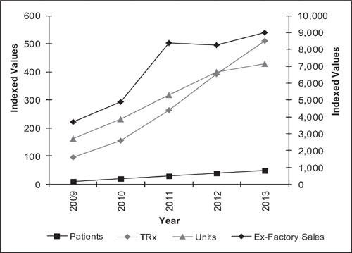
For example, consider the data shown in Figure 4.2. This graph presents the historical data for four different datasets for a single product – patients, total prescriptions (TRx), units and ex-factory sales. Cursory examination of the total prescription trend line suggests that the product growth is accelerating. However, the units dispensed line suggest that the growth is flattening in the market. Focusing on the patient data suggest that the product is growing, albeit at a slower rate than the TRx data suggest. The ex-factory sales line suggests growth, but with an anomalous data point in 2011.
Which interpretation of the data is correct? Why does it appear that the data are in conflict? The explanation depends on the conversion factors derived from the data. Growth of TRx data without a matching growth in unit data suggest that physicians are writing a smaller prescription size – effectively shrinking the number of units dispensed per prescription. The TRx data growing faster than the patient data suggests that physicians are writing more (that is, shorter duration) prescriptions per patient. The spike in the ex-factory sales in 2011 suggests that wholesalers may have speculated in 2011 leading to an increase in ex-factory sales that is not linked to an increase in patient demand. If the forecaster selects only one of these potential data sets the chances for misinterpretation of the market dynamics (and a misguided forecast) are great. The forecaster should use all four datasets and be prepared to explain the changes in market dynamics (conversion rates) that give rise to the seemingly disconnected data trends. The key to forecasting the product is to understand the underlying market dynamics, as evidenced by the illustrative data presented in this example.
Figure 4.2 Historical data for a product
Often a naïve forecaster, or a naïve reviewer of a forecast, will focus exclusively on one dataset. This myopic and dangerous act often will result in erroneous forecasts. However, the other balance point in trending historical data – that of analyzing every conceivable dataset – also can result in a confusion of results. For example, many organizations review weekly prescription data and attempt to forecast these data as an indicator of future product performance. This can be a valuable exercise if the data integrity is strong and the prescription data is representative of the market dynamics (that is, there are no inter-conversion issues related to prescription length or size). However, trending weekly data also can be a very time-consuming exercise for the forecaster and, if the data integrity is weak, can result in erroneous conclusions.
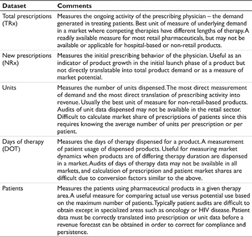
Where then is the balance point for trending historical data? The overarching principle is to use the historical measures that can be most accurately tracked and that best represent historical market dynamics. Significant errors in data reporting will translate into significant errors in trending and forecasting. The integrity of the underlying dataset is paramount. Assuming valid data, at a minimum the forecaster should examine the datasets presented in Table 4.1. These data capture slightly different dynamics in the market that allow the forecaster to triangulate historical activity.
Table 4.1 Data useful in trending historical market dynamics
Two common data elements that have been conspicuously absent from this discussion are market share and product revenue. Both of these datasets are derivatives – that is, market share results from the division of product volume by market volume (where volume may be measured by prescriptions, units, days of therapy, or patients), and product revenue results from the multiplication of product volume by price. Trending either of these two derivative datasets can be misleading and result in erroneous conclusions. For example, if one trends a growth in market share it is impossible to know a priori if this is a result of an increase in product volume (the numerator) or a decrease in market volume (the denominator). These two different dynamics in the market are indistinguishable if only market share is trended. Analogously, trending revenue changes without knowing the change in true price (that is, list price corrected for product mix, discounts, and rebates) clouds the true change in market dynamics. Trending of revenue also involves other issues that will be discussed in the reconciliation and conversion section of this chapter.
As we can see, what seemingly was a straightforward data trending exercise for time-series data involves a judgmental component as well – what is (or are) the best representative historical dataset(s) upon which to form the baseline trend analysis? In the next section we will encounter another judgment call the forecaster must make in performing the statistical trend analyses.
SELECT THE TIME PERIOD FOR TRENDING
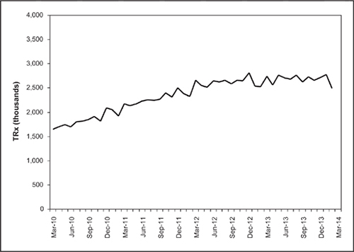
Once the appropriate identity of the datasets to trend has been determined the forecaster then is faced with the question of how many historical data points to include in the trend analysis. Consider the data shown in Figure 4.3, which illustrates performance for a product. The forecaster must select the number of data points to include in the historical trend analysis.
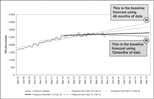
After steady growth from 2010 through 2012, there appears to be a flattening of product performance in 2013. What is the appropriate number of historical data points to use in the time-series trending? Figure 4.4 shows the results of three simple options: trending from March 2010 through February 2014, trending from March 2011 through February 2014, and trending from March 2012 through February 2014 (48, 36, and 24 months of historical data respectively). Inspection of this graph indicates very different projections for 2014 and 2015 depending upon the number of historical data points chosen for the trend analysis. Simple trending algorithms were used for this example, and more complex algorithms may decrease the differences between the trend lines. However, the dilemma of the number of data points to trend remains the same: should the forecaster select a complete dataset or a dataset that is most ‘representative’ of current market conditions?
Figure 4.3 An example of historical product performance
Figure 4.4 Projection using varied historical periods
Statistics and trending software packages can lend insight to this decision … but they may be misleading as well. A naïve view of statistics would tell the forecaster to select the number of historical data points that yields the best ‘fit’ of historical data to the statistical trend analysis (that is, the trend that minimizes root mean square error). In the simplified example above this would be the regression based on 48 months of data. As discussed, this may be the wrong decision is the market events captured in the latest 12 months of data truly represent the environment moving forward – in which case the forecaster must override the statistical best fit and select only 12 months of historical data for the trend analysis. Other statistical techniques – such as moving annual totals or dampening of recent data points – may be used to enhance the statistical outcomes and provide a better ‘best fit’ trend line, but none of these techniques can alleviate the forecaster from the responsibility of making a judgment call on the validity of the historical data. For reviews of in-market forecasts, the first question that should be asked of the forecaster is: ‘How many data points were selected for the time-series analysis and why?’
Once the optimal trend analysis has been established for both the product and the market, the forecaster next turns to quantifying the effect of ex-trend events on these baseline projections.
Applying the Effects of Ex-Trend Events
What are ex-trend events? Simply stated, they are any activities that occur which are not reflected in the historical data. This all-encompassing definition includes events such as government policy revisions, changes in reimbursement environments, evolution in medical treatment paradigms, changes in marketing programs, reallocation of sales resources, adverse publicity, new competition in the market, and so forth. There are a number of ex-trend events that can occur and affect the baseline trend projections discussed in the previous section. The challenge to the forecaster is to identify these events and quantify the effects of the events on the forecast.
Ex-trend events fall into two broad categories – external changes outside the direct control of the company and internal changes governed by the company itself (Table 4.2). The external changes are the result of policy set by external agents – governments, insurers, physicians, public policy organizations, competitors and so forth. Internal ex-trend events are under the control of the company and typically involve changes in marketing and sales strategies for given products and the launch of line-extension products.
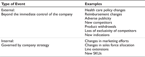
EXTERNAL EX-TREND EVENTS
External ex-trend events include examples such as changes in the regulatory review process in the European Union, the advent of physician drug budgets in Germany, the Affordable Health Care for America Act in the United States, and the rise of internet pharmacy dispensing in Canada. Other examples include publicity in the public domain – such as controversy over suicide associated with certain classes of anti-depressants, safety issues associated with certain weight loss products, product withdrawals due to safety concerns, and so forth. Still more examples arise from the launch of new competing products (or therapies) in the market, the loss of marketing exclusivity for currently marketed products, or patient access to specific health care plans and providers.
Although these examples are very diverse, the general approach for evaluating the effects of these events is to estimate three parameters:
• the magnitude of the effect;
• the timing of the effect; and
• the products affected by the event.
Each of these parameters may be measured using the judgmental techniques discussed in Chapter 2, such as primary and secondary market research data and analog analysis. For some ex-trend events we may need to use scenario analysis to model several alternative outcomes – for example, quantifying the effects of potential pricing changes.
Estimating the magnitude of the effect is akin to peak share analysis – what is the change in forecast product share due to the ex-trend event. The timing of the effect measures the dynamics of the ex-trend event – how quickly will the peak share effect be realized and, if applicable, how quickly will its effects diminish. The last parameter – the products affected by the ex-trend event – enables the forecaster to model disproportionate effects in the market. For example, changes in reimbursement status for a particular class of products may affect all products equally in that class (if they are priced similarly) or may affect some products more than others (presumably the higher-priced products in this example might be more affected than lower-priced products in the same class).
Introduction of New Competitors
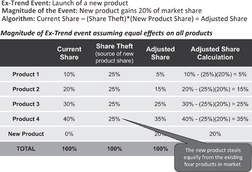
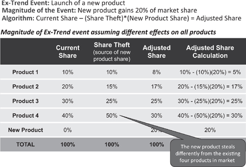
Launch of a new competitor into a market may affect all current products equally or may affect some products disproportionately. These dynamics are captured in the ‘share theft matrix, as illustrated in Figures 4.5 and 4.6 for the entrance of a new competitor that is expected to garner 20 percent market share. In Figure 4.5 the competitor steals equally from all products in the market. In Figure 4.6 the competitor steals disproportionately from products in the market – taking its greatest share from the products that presumably have the greatest degree of similarity to the new entrant.
Figure 4.5 Share theft matrix illustrating equal effects from a new competitor
Figure 4.6 Share theft matrix illustrating disproportionate effects from a new competitor
The above figures demonstrate the method for estimating the effects of the new competitor on in-market product shares, but how does the forecaster measure the magnitude of the new competitor market share (for example, the 20 percent share assumed for the new product in Figures 4.5 and 4.6). This is accomplished using the new product forecasting techniques discussed in Chapter 3, where the new product share and adoption may be modeled using the various share and adoption curve techniques presented in this prior chapter.
There is one specific case of new competitor introduction for which we have good analog data in the United States – namely, the introduction of a generic product into the market. In this case, the generic product essentially is the new competitor introduced into the market. Using the share theft matrix discussed above the forecaster may readily estimate the effects of the generic introduction. In a majority of historical cases the effect of the generic product has been to gather share disproportionately from the branded product of the same active chemical composition. Use of the share theft matrix allows the forecaster to model this dynamic or, if appropriate, effects on the shares of other products in the market.
INTERNAL EX-TREND EVENTS
Internal ex-trend events are those activities under the direction of the company itself. These include activities such as the introduction of line extensions, changes in marketing strategies and programs, and changes in sales force resource allocation. Decisions taken by the organization regarding these activities affect future product trends.
Line Extensions
Line extensions are products based on changes to currently marketed products, for example, a new dosing schedule or a new formulation of an existing product. Changing from a twice-daily dosing to once-daily dosing, or introducing an aqueous (as opposed to non-aqueous) formulation of an intranasal spray are both examples of line extensions. The goal of a line extension is to provide therapeutic benefits to the patients from the new dosing schedule or formulation. An added benefit for a company occurs when the line extension carries marketing exclusivity beyond that offered by the original formulation, or if the line extension is marketed at a higher price than the original formulation. These dynamics were discussed in detail in the ‘cannibalization’ section of Chapter 3.
The previous chapter also discussed methods for line extension forecasting, treating the line extension as a new product introduced into the market. In some cases line extensions also may be forecast using the ex-trend methodologies discussed here. If these methodologies are employed, the effect of the line extension on the in-market product is analogous to that of a new competitor entering the market and having a disproportionate effect on the currently marketed formulation. In essence, the techniques used for evaluating new competitor effects on the in-market product may be used in the forecast.
Line extensions present a unique challenge to the forecaster. The line extensions may be forecast using the new product techniques discussed in Chapter 3
Stay updated, free articles. Join our Telegram channel

Full access? Get Clinical Tree


