The Zurich HF2IS Impedance Spectroscope (Zurich 2015) is the measurement equipment which was used in this measurement. The HF2IS is used to excite the subject and measure the EBI datasets from the subject through sense electrodes. The HF2IS is connected to the switch-box through connector cables.
The HF2IS was limited to two channels (Channel 1 and 2); because of this, at any given time four electrodes (two electrodes from each channel (Excitation A and B)) were used to excite the subject and four electrodes (two electrodes from each channel (Sense A and B)) were used to sense the EBI data. Thus, eight electrodes are active at a time. These channels are shown in Fig. 4.1.
The sensed (measured) EBI datasets were stored in a computer for further analysis. The attached computer is also used to control the switch-box and HF2IS impedance spectroscopy equipment.
A program developed at T.J. Seebeck Department of Electronics was used to control the switch-box that switches/selects the electrodes’ configuration for each time-step automatically. Nevertheless, the configuration of the electrode can also be set up by the advanced user.
In order to make the simple representation of EBI dataset, it is assumed that the EBI data is the summation of the following four components:

where (S ICG ) and (S IRG ) are the cardiac and respiratory signals, respectively, (S Artefact ) is unwanted motion artefact caused by body movements or muscle activity, and (S Noise ) is noise.

(4.1)
The heart rate S ICG (Eq. 4.1) of a healthy person can vary in the range between 60 and 240 bpm (1–4 Hz), and the respiration rate S IRG (Eq. 4.1) of a healthy person can vary from about 12–30 breaths/min (0.2–0.5 Hz) (Mughal 2014).
4.1.2 Waveforms and Spectra of the EBI Signals
The waveform of the cardiac and respiratory components of the EBI signal are relatively smooth (Min et al. 2000); that is why only a few higher harmonics are required for representing them. Figure 4.2 shows the measured and filtered IRG signal from measured EBI, which corresponds to the subject’s respiration, as well as the ICG signal, which corresponds to the cardiac activities of the subject.
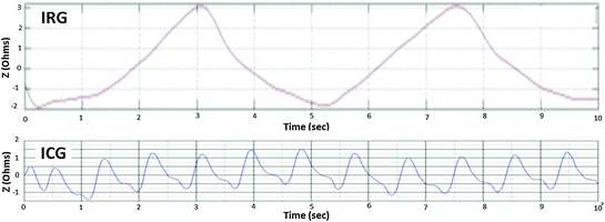

Fig. 4.2
Two cycles of respiration and ~12 cycles of cardiac activity in 10 s
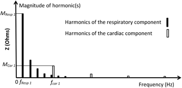
Unfortunately, muscular activities also lie on the same frequency range as that of the cardiac signal, and the higher harmonics of the respiratory signal also lie on the same frequency range of the cardiac signal, as shown in Fig. 4.3 (Mughal 2014).
A simplified possible sketch of the harmonic spectrum of the EBI signal is shown in Fig. 4.3. The possible spectrum is sketched for the signal components shown in Fig. 4.2; in the spectrum, it is illustrated that the fifth harmonic of the respiration signal is partially overlapping with the first harmonic of the cardiac signal, and that the other higher harmonics of the respiration signal “enter” the cardiac signal frequency range.
Based on the literature survey and analysis of the existing thorax impedance models, as well as the origin of the ICG signal (Sect. 2.4 of Chap. 2 and in our published paper (Mughal et al. 2014)), it is assumed that none of the existing models are accurate enough to imitate the real phenomena of the ICG signal. Based on these limitations, it was therefore decided to use the 16-electrode configuration belt to measure the ICG and IRG signals instead of one of the existing models. The candidate existing configurations of electrodes are discussed in Sect. 2.4.4 of Chap. 2. The curve-fitting method is used to model the measured signals.
With this approach, these signal models would be more realistic and the underlying model parameters would be easily tuneable.
The models and evaluation methods are discussed below in Sect. 4.2. In what follows, the four measured EBI datasets and the clean ICG and IRG datasets are used.
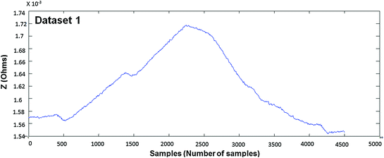
In Figs. 4.4, 4.5, 4.6, 4.7, 4.8 and 4.9 (Datasets 1–6), each dataset has been measured from different positioning of electrodes. Our results are published in Mughal et al. 2014.
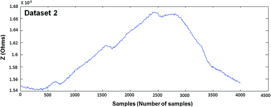
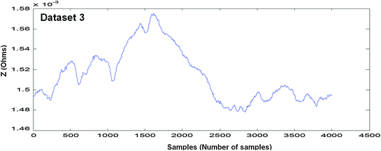
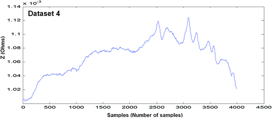
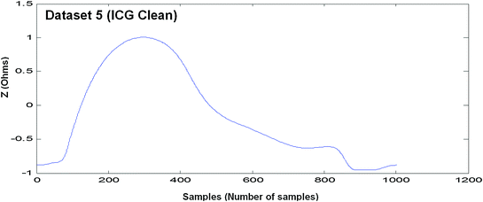
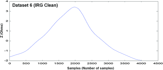

Fig. 4.5
Measured EBI waveform (Dataset 2)

Fig. 4.6
Measured EBI waveform (Dataset 3)

Fig. 4.7
Measured EBI waveform (Dataset 4)

Fig. 4.8
Measured EBI waveform (Dataset 5)

Fig. 4.9
Measured EBI waveform (Dataset 6)
4.2 Method for Modelling the Bio-Impedance Signal
Modelling of the EBI signals can be performed by way of using template signals. This is discussed in Chap. 3 (Fig. 3.1) and Sect. 3.2 (Modelling and Building Simulator, Step 5 of Fig. 3.2).
Here the curve-fitting method is used to model the ICG and IRG signals.
Different curve-fitting models are evaluated by comparing the measured and modelled signals based on statistical parameters and visual fit.
4.2.1 Curve-Fitting Method
In the curve-fitting method, three different curve-fitting models are compared, namely polynomial, Fourier series, and sum of sines. The comparison criteria were based on visual fit and statistical parameters, namely sum of square error (SSE), correlation between the model and the corresponding dataset fitted modelled values (R-Square), and execution time. Each curve-fitting method and statistical parameters are discussed and evaluated below (Mughal et al. 2015a):
4.2.1.1 Models and Evaluation Method
Each model is discussed and evaluated with the help of six EBI measured datasets. Four datasets are raw EBI measured datasets and two are cleaned ICG and IRG signals.
(a) Polynomial Model
Polynomials are well suited for cases where a fairly simple empirical model is needed; they can be used for interpolation or extrapolation to characterize data by means of a global fit. The general polynomial model formula is given in Eq. 4.2:

where n is the degree of the polynomial (highest power of the predictor variable), n + 1 is the order of the polynomial (number of coefficients), p i is the coefficients, and t is time.

(4.2)
In this work, the polynomial model was evaluated for degrees 1–9 for the four EBI datasets; degree 9, which is the highest order available in the toolbox, gave the most suitable results. The comparative results are shown in Table 4.1 and Figs. 4.10, 4.11, 4.12, 4.13, 4.14 and 4.15.
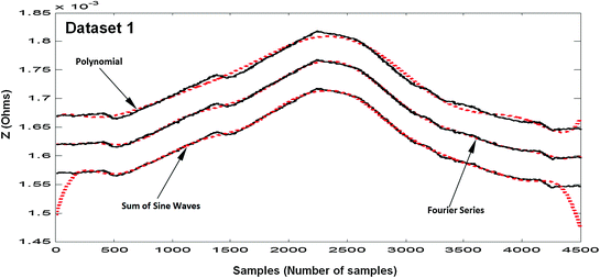
Table 4.1
Evaluation criteria results for the modelled signals
Datasets | Sum of sine waves (24 coeff) | Fourier (18 coeff) | Polynomial (10 coeff) | |||||||
|---|---|---|---|---|---|---|---|---|---|---|
SSE | R–Sq | SSE | R–Sq | SSE | R–Sq | SSE Avg | SSE Min | SSE Max | R–SqAvg | |
Dataset 1 | 1.0424e-07 | 0.9917 | 0.1612e07 | 0.9987 | 1.2270e-07 | 0.9903 | 0.810e-07 | 0.161e-07 | 1.23e-07 | 0.9935 |
Dataset 2 | 0.9044e-07 | 0.9875 | 0.1786e-07 | 0.9976 | 0.3050e-07 | 0.9959 | 0.463e-07 | 0.179e-07 | 0.904e-07 | 0.9936 |
Dataset 3 | 1.9417e-07 | 0.9274 | 0.6476e-07 | 0.9758 | 1.3185e-07 | 0.9506 | 1.326e-07 | 0.6476e-07 | 1.9417e-07 | 0.9512 |
Dataset 4 | 0.8054e-07 | 0.9714 | 0.3506e-07 | 0.9876 | 1.6683e-07 | 0.9409 | 0.941e-07 | 0.3506e-07 | 1.6683e-07 | 0.9666 |
SSE Avg, R-Sq Avg | 1.17e-07 | 0.970 | 0.335e-07 | 0.9758 | 1.13e-07 | 0.969 | 0.879e-07 | 0.9762 | ||
SSE Min, R-Sq Min | 0.805e-07 | 0.161 | 0.161e-07 | 0.9758 | 0.305e-07 | 0.941 | 0.161e-07 | 0.9512 | ||
SSE Max, R-Sq Max | 1.94e-07 | 0.9917 | 0.648e-07 | 0.9987 | 1.67e-07 | 0.996 | 1.9417e-07 | 0.9936 | ||
Clean ICG Signal with different scale | ||||||||||
Clean ICG | 0.1996 | 0.9994 | 0.0611 | 0.9999 | 2.8229 | 0.9937 | 1.0279 | 0.0611 | 2.8229 | 0.9959 |
Ex. Time (s) | ~49.170 | ~4.694 | ~3.419 | |||||||
Clean IRG Signal with different scale | ||||||||||
Clean IRG | 7896.1e-07 | 1 | 2890.6e-07 | 1 | 19.5782 | 0.9983 | 6.5264 | 2890.6e-07 | 19.5782 | 0.9994 |

Fig. 4.10


Results of fitting of the EBI dataset 1: the measured dataset 1 (solid lines, black) and fitted models (dotted lines, red) (Mughal et al. 2015a). Results for the sum of sines waves model are presented without offset. For readability, the results for Fourier series model are offset by 0.05 × 10⁻³, and the results for Polynomial model are offset by 0.1 × 10⁻³
Stay updated, free articles. Join our Telegram channel

Full access? Get Clinical Tree


