(1)
Physical Chemistry, Department of Chemistry, Munich Center for Integrated Protein Science (CiPSM) and Center for Nanoscience (CeNS), Ludwig-Maximilian-Universität München, Munich, Germany
(2)
Loomis Laboratory of Physics, Department of Physics, University of Illinois at Urbana-Champaign, Urbana, IL, USA
Abstract
Pulsed interleaved excitation (PIE) employs pulsed laser sources that are interleaved such that differentially colored fluorophores can be measured or imaged quasi-simultaneously in the absence of spectral crosstalk. PIE improves the robustness and reduces data analysis complexity of many fluorescence techniques, such as fluorescence cross-correlation spectroscopy (FCCS) and raster image cross-correlation spectroscopy (ccRICS), two methods used for quantitative investigation of molecular interactions in vitro and in living cells. However, as PIE is most often used for fluorescence fluctuation spectroscopy and burst analysis experiments and utilizes time-correlated single-photon counting detection and advanced optoelectronics, it has remained a technique that is mostly used by specialized single-molecule research groups. This protocols chapter provides an accessible overview of PIE for anyone considering implementing the method on a homebuilt or commercial microscope. We give details on the instrumentation, data collection and analysis software, on how to properly set up and align a PIE microscope, and finally, on how to perform proper dual-color FCS and RICS experiments.
Key words
Pulsed interleaved excitationRaster image correlation spectroscopyTime-correlated single-photon countingFluorescence cross-correlation spectroscopyFluorescence correlation spectroscopyConfocal laser scanning microscopyFCSFCCSRICSccRICSCLSM1 Introduction
Fluorescence cross-correlation spectroscopy (FCCS) and raster image cross-correlation spectroscopy (ccRICS) are very powerful fluorescence fluctuation spectroscopy (FFS) techniques for investigating dynamics, concentrations, and molecular interactions of fluorescently labeled biomolecules in vitro and in living cells [1, 2]. FCCS is the dual-color extension of fluorescence correlation spectroscopy (FCS), the technique with which dynamics and absolute concentrations of diffusing molecules are determined from point fluorescence fluctuation spectroscopy measurements by temporal autocorrelation analysis [3]. ccRICS is the analogous extension of the raster image correlation spectroscopy (RICS) method, the technique with which dynamics and absolute concentrations of diffusing molecules are determined from fluorescence fluctuation imaging experiments by spatial autocorrelation analysis [4, 5]. However, due to spectral crosstalk of commonly used fluorophores for FFS, FCCS and ccRICS suffer from a relatively low sensitivity in terms of measuring interactions. Under some circumstances, it is possible to correct experimental data a posteriori for crosstalk [6, 7]. Quantitative analysis of molecular interactions inside living cells with FCCS in the presence of considerable crosstalk has been shown to be possible, but requires complex and careful data analysis [8, 9]. Therefore, it is desirable to avoid crosstalk altogether to reduce complexity and increase robustness of data analysis.
Pulsed interleaved excitation (PIE) was based on the earlier work of Kapanidis and co-workers [10] and was originally developed to avoid problems of spectral crosstalk during FCCS experiments and to provide stoichiometry information from burst analysis experiments [11]. In addition, PIE can be used to increase the robustness of many quantitative fluorescence techniques. For example, it allows the Förster resonance energy transfer (FRET) efficiency to be calculated directly from FCCS experiments without a priori knowledge of the labeling degree [11], it increases the accuracy of single-pair FRET experiments with multiparameter fluorescence detection [12], it allows for quantitative fluorescence fluctuation and lifetime imaging [13], and it is commonly used in dual-focus FCS for accurate measurements of the diffusion coefficient [14]. At present, many biological systems have been studied using PIE; for an overview, see ref. 15.
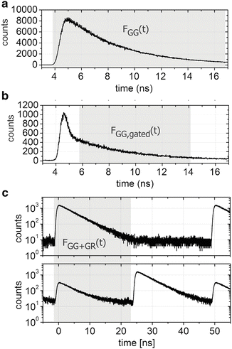
PIE is typically performed in combination with time-correlated single-photon counting (TCSPC) detection, a technique in which the time delay of a detected fluorescence photon is measured relative to the laser excitation pulse (of a duration typically ≲100 ps) with extremely high temporal resolution [16]. When using TCSPC, fluorescence is typically measured on two timescales: the macroscopic timescale, or “macrotime”, that is, the arrival time of the photons with respect to the start of the experiment with a time resolution of typically 30–100 ns, and the microscopic timescale, or “microtime,” which is the time between the excitation pulse and emission of the detected photons with a time resolution of a few ps (see Fig. 1a). A histogram of the photon microtimes in a TCSPC experiment can be used for analyzing the fluorescence lifetime (see Fig. 1b) while the macrotime traces can be used for, inter alia, autocorrelation analysis (see Fig. 1c). When TCSPC is combined with confocal laser scanning microscopy (CLSM), confocal images can be constructed from the macrotimes (see Fig. 1d). The “trick” used in PIE lies in the fact that, in addition to just employing two (or more) pulsed lasers and two (or more) detectors, the lasers are perfectly synchronized with a time delay between them that is smaller than the repetition period of the lasers, i.e., they are interleaved. This creates a new, temporal separation of emitted photons in addition to their common spectral and spatial separation. Indeed, as illustrated in Fig. 1e for a two-color PIE microscope, crosstalk of the green fluorophore into the red detection channel is temporally well separated from direct emission of the red fluorophore when the delay between the two lasers is set appropriately. By setting defined time gates [17] in the microtime histograms, species-specific macrotime traces and/or images can be constructed (see Fig. 1f, g).
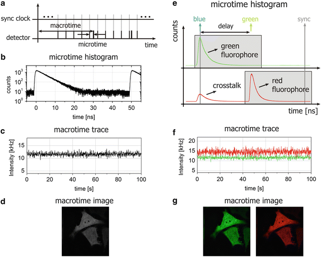
Fig. 1
Illustration of TCSPC and PIE. (a) The basic principle of TCSPC is shown where both the macro- and microtime of each detected photon are recorded in the experiment. (b) By histogramming the microtimes of all detected photons, the fluorescence decay of the fluorophore is observable. (c) By consecutive binning of the macrotimes of the detected photons, an intensity or macrotime trace is obtained. (d) When recording data with a CLSM, the macrotimes of the TCSPC data can be binned into image pixels and in this way the confocal image can be displayed. (e) Illustration of a two-color excitation two-color detection PIE experiment with TCSPC detection. The selected time gates for further analysis are hatched in gray. Species-specific macrotime traces (f) and images (g) can be calculated from the macrotimes of the photons within the selected time gates. As there is no crosstalk in the macrotime images, the clear signal in both channels indicates that both fluorophores are present in the imaged cells
Nowadays, the PIE technique is accessible to a large scientific community. Commercial ready-to-use point-measurement PIE microscopes exist that allow i.a. FCCS experiments with PIE. PIE can also be integrated into commercial CLSM systems (see Note 1), introducing quantitative fluorescence fluctuation analysis (i.a. FCCS and cross-RICS) and multicolor fluorescence lifetime imaging (FLIM) capabilities into the system. Upgrading an existing CLSM can be advantageous because it can be both time and cost saving when the microscope is already present. Moreover, most, if not all, functionalities of the microscope can subsequently be used in combination with PIE. Different TCSPC hardware manufacturers provide ready-to-use hardware upgrade “kits” for commercial CLSMs and additionally offer excellent technical support, avoiding the need for experience with assembling advanced optics and electronics. Finally, building ones’ own PIE system also has its advantages: the microscope can be specifically designed to the researchers’ needs, usually costs significantly less than a commercial system, and can be modified and upgraded in a straightforward fashion. It does, however, require expertise in assembling microscopes.
Although PIE is available commercially, to date it has been employed mostly by specialized single-molecule research groups. This is due, in part, to the required expertise in fluorescence correlation spectroscopy (FCS), TCSPC, and microscopy, if a PIE microscope is to be built ab initio. To make PIE more easily accessible, we have written this chapter as a step-by-step guide for the correct implementation and application of PIE, be it on a completely homebuilt setup or on an upgraded commercial CLSM. We give a comprehensible overview of the instrumentation, data collection, and analysis software that is suitable for PIE, discuss how to properly set up the excitation and detection equipment, give advice how to align a PIE microscope for optimal performance, and finally, give a detailed protocol for doing point-based and image-based measurements and subsequent PIE-FCCS and PIE-RICS analyses. Our hope is that by reading this chapter, nonexpert research groups interested in PIE will finally take the step to implement it, thereby profit from the benefits, possibilities, and robustness that PIE offers.
2 Materials
2.1 Instrumentation
1.
Lasers: For pulsed interleaved excitation, pulsed laser sources are required. In principle, picosecond (ps)-pulsed lasers with high output stability and preferentially collimated, TEM00 output are well suited for PIE (see Note 2). Most importantly, all lasers that are used simultaneously need to be synchronized (see Subheading 3.1). It is possible to use continuous-wave lasers and modulate the intensity using an acousto-optically modulated (AOM) as was performed in the original report of PIE, but at the cost of losing the fluorescence lifetime information [11]. Nowadays many suitable lasers are available, such as (but not limited to):
Externally triggered ps-pulsed quasi-monochromatic diode lasers covering a wide range of the visible spectrum.
Fixed-frequency or externally triggered ps-pulsed white-light supercontinuum lasers providing ultimate flexibility in the choice of excitation wavelengths.
Fixed-frequency fs–ps-pulsed tunable fiber lasers covering the visible spectrum and providing extremely high spectral purity.
An AOM-modulated CW laser [11].
As the lasers need to be synchronized, only one fixed-frequency laser can be used in a PIE microscope at the most, while all other lasers should be synchronized by external triggering. The laser power requirements for PIE are similar as for normal FCS experiments, i.e., roughly 1–100 μW per laser, as measured at the sample, should be sufficient for most applications. Because of losses in combining the lasers, coupling them into the single-mode fiber and then into the sample, the power output of the laser should be significantly more than 100 μW. For most applications, an average laser output power of 1 mW is more than sufficient.
2.
Electronic delay box: The electronic delay box introduces a variable delay in an electrical signal. We use electronic delay boxes to both shift the laser pulses with respect to each other and adjust the arrival time at the TCSPC hardware of the signal from the detectors. Delay boxes are not necessary for PIE, but are extremely convenient. In our case, the delay boxes are homebuilt and can delay signal in steps of 1 ns from 1 to 32 ns.
3.
Attenuators: Lasers can be attenuated manually by partially blocking the beam path (see Note 3) or with a neutral density filter or electronically with an acousto-optical tunable filter (AOTF). An AOTF has the advantage that different lasers can be attenuated independently and in an automated fashion.
4.
Single-mode (polarization maintaining, see Note 4) optical fibers: Different lasers should be combined into a single fiber (see Note 5) and a broadband achromatic collimator should be used to collimate the light into a free beam again before directing the light to the microscope (see Note 6). Optical fibers can also be used to delay pulses optically (see Note 7).
5.
Optics: In general, highest-quality, antireflection-coated optics should to be used. More specifically, silver mirrors provide high reflection in the visible spectrum but are difficult to clean. Achromatic doublet lenses minimize optical aberrations. Di-/polychroics, excitation and emission filters should have sharp cut-in/cut-out and a high degree of reflection and/or transmission (see Fig. 2b). Thicker substrates for the polychroics are desirable to avoid astigmatism in the beam (see Note 8). Excitation filters are only needed if the laser is not monochromatic. Emission filters additionally should block all excitation wavelengths by at least OD6 and higher if measuring on surfaces where a higher fraction of laser light is reflected into the detection path.
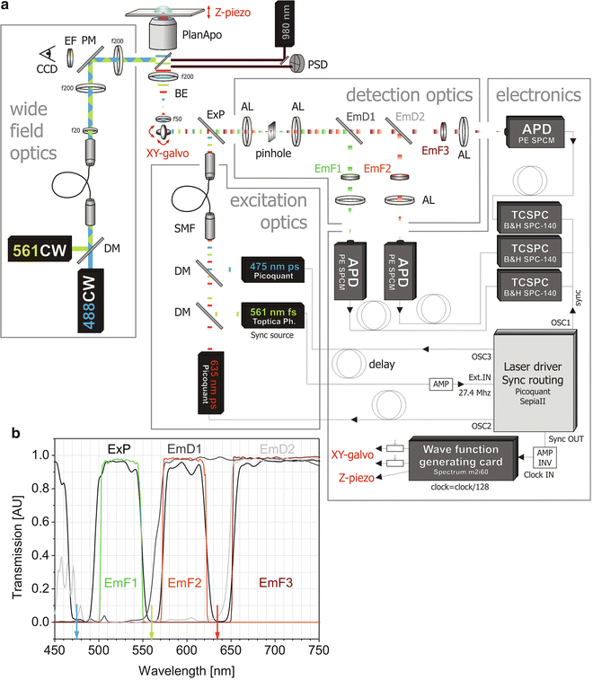
Fig. 2
Schematic illustration of our 3-color PIE microscope. (a) A frequency-doubled Erbium-doped fiber laser pulsing at 27.4 MHz determines the clock of the whole system. A fraction of its 561-nm output is converted to an electrical signal and fed to the laser driver of the 475-nm and 635-nm lasers that are consequently synchronized to the same frequency. A variable electronic delay box delays the latter two lasers with respect to the 561-nm laser for proper 3-color PIE. Three independent TCSPC devices, each connected to an avalanche photodiode (APD) detector, and an arbitrary wave-function generating PCI card controlling the galvo and a Z-actuator, are synchronized with the master clock through the laser driver. Abbreviations: ExP = excitation polychroic mirror, EmF1–3 = emission filters, AL = achromatic lens, BE = beam expander, DM = dichroic mirror, EmD1-2 = emission dichroics mirror, SMF = single-mode fiber. (b) Spectrum of the optical elements for filtering on the PIE microscope. The excitation polychroic efficiently reflects the three laser lines depicted with an arrow, while maximally transmitting the emission light. After the pinhole, the emission dichroics furthermore separate the emission into three large spectral windows, and the emission filters define the specific spectral detection windows
6.
Fast mirror scanner: When scanning is desired, scanning mirrors will need to be incorporated into the system. Different types exist, but for most imaging applications, two closely spaced galvanometric mirrors, or “galvo,” are sufficient. Depending on the manufacturer and controller electronics used, the position of the galvo can be controlled via an analog signal or digitally. A feedback control can be used for calibration purposes, but is generally not needed during imaging experiments. Of importance, a resonant mirror allows for higher imaging speeds, but does not allow specific positioning of the point spread function (PSF) without physically moving the sample.
7.
Kepler-type telescope: To maximize the scanning speed, the size of the galvo mirrors needs to be kept to a minimum. Hence, it is often desirable to expand the beam after the scanner to fill the back aperture of the objective (see Note 9). In addition, the focal plane of the mirrors needs to be imaged on the back aperture of the objective to ensure the excitation beam is constant during scanning. To do this, a telescope is placed between the scanner and the objective. We use two achromatic planoconvex lenses mounted in a cage for stability (see Note 10).
8.
Microscope base: For a homebuilt PIE microscope, any microscope base can be used. It is important that 100 % of the light can be directed to the port where the detection optics are mounted. Microscopes with more available input ports also allow more functionality to be incorporated into the system.
9.
Objective lens: The objective is the heart of the confocal microscope and only the best quality objectives should be used. High-NA water (NA ≥ 1.2) or oil (NA ≥ 1.3) immersion objectives with corrections for chromatic and/or spherical aberration (see Note 11) and with a correction collar for coverslip thickness and/or refractive index (n-) mismatches are desirable (see Note 12).
10.
Immersion solution: For long measurements using a water-immersion objective, nonvolatile immersion liquids with n = 1.33 should be used.
11.
Z-actuator: To control the focus of the sample, a Z-actuator can be incorporated into the setup. Either the sample or the objective can be mounted on a Z-actuator. The Z-actuator is usually a piezoelectric element with subnanometer resolution.
12.
Pinhole: A 50–100-μm diameter pinhole works best for most applications. For multicolor detection, a single pinhole is sufficient for defining the confocal volume and the different colors can be separated after the pinhole. In general, a larger pinhole results in a higher apparent molecular brightness at the cost of a slightly larger PSF (see Note 13 and ref. 18).
13.
Detectors: Single-photon counting detectors (see Note 14) are connected to the TCSPC device via an electronic delay box. The detection path after the pinhole should be completely enclosed in a light-tight container of some sort (a box or tubes) to shield the sensitive area of the detectors from stray light.
14.
TCSPC device: To optimally use the lifetime information available from pulsed excitation, TCSPC detection is desired. Preferably, each detector should be connected to an independent TCSPC device to avoid dead time related artifacts (see Note 15).
15.
Router: If necessary, a router can be used at low count rates. A router allows multiple detectors to be connected to the same TCSPC device. This device sends digital detector routing bits along with the photons to the TCSPC device (see Note 15).
16.
Trigger: To ensure that all electronics are synchronized, an external trigger is needed to start the measurement. This can be done with a simple DAQ device that sends out a TTL pulse when the experiments begins, which ensures all TCSPC devices start measuring simultaneously.
17.
Widefield optics: When performing cellular experiments, it is useful to have a widefield module on the microscope. In this way, cellular fluorescence can be observed directly through the eyepiece or on a camera, making it quick and easy to select cells with appropriate expression levels for the confocal measurements.
2.2 Sample Preparation
1.
Sample holder: To avoid evaporation of the sample at small volumes and to protect the sample from contaminations, a closed-lid sample holder is preferred. Be sure the coverslip thickness matches the specifications of the objective (see Notes 16 and 17).
2.
Fluorophores for PIE: Suitable properties of fluorophores used in PIE experiments are good photostability, no significant spontaneous degradation, little or no fast photophysics, negligible nonspecific absorption and good solubility. Many organic dyes exist that possess all these properties. If photostability or fast photophysics are a concern, such as when using fluorescent proteins, combining PIE with fast CLSM imaging provides an excellent alternative to point measurements [13].
3.
Reference dyes: To calibrate the system and check the sensitivity, reference dyes with known diffusion coefficients (D) should be used. Be aware that the D of dyes depends significantly on their functionalization [19]. In our experience, ATTO488 carboxylic acid (ATTO-TEC GmbH, Siegen, Deutschland), Rhodamine B and ATTO655 carboxylic acid (ATTO-TEC) perform very well as reference dyes for 475-nm, 561-nm and 635-nm excitation respectively (see Note 18).
4.
Buffers: Care needs to be taken that the buffers used exhibit as little autofluorescence as possible. This can be particularly challenging when the buffer contains a number of salts. In vitro experiments can be performed with sample volumes as small as 10–20 μL (see Note 19).
2.3 Acquisitioning and Analysis Programs
1.
Acquisitioning software: For a homebuilt PIE microscope, no special acquisitioning software is needed beyond the manufacturer’s software to control the TCSPC hardware when only point-based measurements are performed. When imaging with PIE is to be performed on a commercial CLSM, usually the manufacturer’s software, together with the software controlling the TCSPC hardware are used to acquire images. For our homebuilt CLSM, we use an acquisitioning program written in the C# programming language to control and synchronize the galvo and TCSPC cards and to provide a user interface for displaying PIE images in real time (see Note 20).
2.
Point-analysis software: Packages for analysis of experiments with PIE are available from different manufacturers. We use an in-house developed program, PIE Analysis with Matlab or simply “PAM.” With PAM, the following analysis methods can be applied to PIE data: individual and global FCS/FCCS analysis (see Subheading 3.4), fluorescence lifetime correlation spectroscopy [20], brightness analysis by photon counting histogram [21] or cumulant analysis [22], pair correlation analysis [23], line/circle scanning FCS [24, 25], single-pair FRET by burst analysis and multiparameter fluorescence detection (MFD) [26, 27], photon distribution analysis [28], fluorescence lifetime analysis and time-resolved anisotropy analysis. In addition, various Monte-Carlo simulation algorithms are available.
3.
Image-analysis software: We also have an in-house developed program for CLSM image analysis, called Microtime Image Analyzer or “MIA.” With MIA, the following analysis methods can be applied to PIE imaging data: individual, global and lifetime-weighted raster image correlation spectroscopy [29] (see Subheading 3.4), number and brightness analysis [30], phasor analysis [31] and fluorescence lifetime imaging.
3 Methods
3.1 Setting Up PIE Excitation Equipment
The first step in using a PIE microscope is setting up the excitation equipment according to the type and number of fluorophores under investigation as well as their fluorescence lifetime. Be sure to be well acquainted with laser safety before proceeding with any steps involving lasers.
1.
Master clock: A master clock is needed to synchronize the instrumentation. This is typically taken as the frequency at which one of the pulsed lasers is run. We illustrate in Fig. 2 how the frequency of a fixed-repetition rate laser is used as the master clock for all other lasers, as synchronization source for the TCSPC hardware, as well as for the wave-function generating card controlling the galvo and Z-actuator. The system shown in Fig. 2 is a schematic of our actual three-color PIE microscope.
2.
Frequency: The number of excitation lines determines the repetition period (and thus frequency) of the lasers (see Fig. 3a and Note 21), and conversely, a fixed-frequency laser determines the maximum number of fluorophores that can be imaged optimally and simultaneously with PIE. Keep in mind that the molecular brightness (in Hz) will decrease at lower repetition frequencies [11].
Fig. 3
Laser settings for PIE. (a) Schematics showing the synchronized, interleaved laser pulses on the nanosecond timescale. The more excitation lines in a single PIE experiment, the lower the repetition frequency needs to be for each, as illustrated for a two-color (left) and three-color (right) PIE setup. (b) Since TCSPC detection is used, the fluorescence lifetime of each fluorophore is available in a PIE experiment, as illustrated for a two-color excitation, two-color detection PIE microscope. The green fluorophore, excited with the green laser, will emit primarily in the green detection channel with a residual, though non-negligible spectral bleedthrough into the red detection channel. The red fluorophore, excited with the red laser, will emit only in the red detection channel. The delay of different lasers determines the performance of the PIE setup. By setting the delay of the red laser correctly (25 ns, left panels), bleedthrough and direct emission of the red fluorophore can be perfectly separated temporally, while, for a too short delay of the red laser (10 ns, right), temporal overlap of the green signal after green excitation into the red detection channel with red excitation will occur
3.
Delay: The delay between laser pulses should be set according to the fluorescence lifetime of the previously excited fluorophore, as illustrated in Fig. 3b for two-color excitation, two-color detection. For externally triggered lasers, the delay can be set with an electronic delay box between the laser driver and laser head. For lasers that cannot be triggered electronically, a delay can be set with an optical fiber (see Note 7) or a free-beam delay line.
4.
Pre-/post-fiber separation: After adjusting the delay time, combine all lasers into a single fiber (see Notes 5 and 22). A factory prealigned beam combiner can also be used to combine fiber-coupled lasers into one single-mode fiber when the excitation path is not changed regularly. This approach has the advantage that no pre-fiber alignment is necessary once the excitation path is set up.
5.
Power: Depending on the experiment, a laser power between 0.1 and 100 μW in the sample is needed. Use attenuators to achieve the proper laser power (see Note 23).
There are some important considerations related to the excitation module when upgrading a commercial CLSM to PIE.
6.
For convenience and safety, lasers for PIE should be combined in a single, closed laser combining unit.
7.
The necessary excitation polychroic has to be installed in the microscope.
8.
Usually, an extra single-mode fiber input is available on the CLSM that can be used to couple in the PIE lasers. Alternatively, the PIE lasers can also be combined with existing lasers in the same fiber, if no extra input port is available.
9.
The timing (master clock, frequency, delay) and power of the PIE lasers is usually controlled independently of the CLSM software.
3.2 Setting Up PIE Detection Equipment
Next, the detectors and TCSPC hardware need to be set up for PIE experiments. It is important to be well acquainted with the dos and don’ts of TCSPC hardware, so we suggest referring to the manufacturers’ manual before proceeding in this section.
Get Clinical Tree app for offline access

1.
Emission optics: Choose and install the emission optics according to the spectra of the fluorophores to be used for the experiments (see Notes 24 and 25).
3.
Detectors: On a homebuilt microscope, the detectors need to be connected to the TCSPC hardware, provided their output signal has the correct amplitude and polarity. Also the delay between photon detection and recording of the TTL pulse by the TCSPC card should be similar for all detectors. On a commercial CLSM with photon counting detectors, the output of the detector can be split with one input directly connected to the external TCSPC hardware and the other to the detector input of the CLSM. When appropriate detectors are not available within the CLSM, a fiber-based output of the LSM unit can be used to guide the emission light to a light-tight single-photon counting detection box that carries the emission optics, detectors and TCSPC hardware.
4.
Galvo synchronization: On a homebuilt microscope, the TCSPC and galvo hardware can usually be controlled in sync by letting the master clock control the galvo, as is the case on our PIE setup (Fig. 2). On a commercial CLSM, the galvo operates independently from the PIE hardware, creating the need for another means of synchronizing the detected signal and location of the excitation spot. Most often, the galvo hardware transmits a digital signal to the TCSPC hardware containing pixel, line and/or frame bits during image scanning. These bits can be written directly into the recorded photon files as pseudo-photons, which allows a posteriori histogramming of photons into the individual pixels in an image. For more information regarding synchronization of the galvos, it is advisable to contact the manufacturer of the microscope (see Note 27).
5.
Count rate: Fluctuation techniques analyze fluctuations in fluorescence intensity and, as such, are performed at very low concentrations. Under normal conditions, the single-to-noise ratio of a FCS experiment depends on the molecular brightness of the fluorophore but is independent of concentration within certain limits [11]. Hence, it is not necessary to measure at high count rates (>500 kHz). For some applications, such as accurate fluorescence lifetime or brightness measurements, it is even recommended to measure at low (1–100 kHz) count rates (see Notes 15 and 27).
6.
PIE channels: Because of the microtime information available with TCSPC detection, analysis of PIE data can be performed with subsets of photons in a single detection channel. This is done by setting a defined microtime gate or “PIE channel” [17]. PIE channels add an extra dimension for data analysis (see Subheading 3.4). At high count rates, the PIE channel can usually be set to encompass the complete fluorescence decay of a fluorophore (Fig. 4a). With two-color PIE, PIE channels allow green fluorophore crosstalk to be separated from red fluorophore direct emission. At lower count rates, scattering will likely contribute significantly to the signal; a narrower time gate can then be used to increase the SNR of the measurement by omitting the scattering photons from the PIE channel (Fig. 4b). Finally, since different detectors are usually used for PIE, it can be beneficial to simply combine the photons from different PIE channels (Fig. 4c). For example, the crosstalk of the green fluorophore on the red detector can be combined with its direct emission on the green detector to increase the SNR when direct excitation of the red fluorophore with green light is insignificant.