(1)
Department of Mathematics, University of Florida, Gainesville, FL, USA
14.1 Introduction to Immuno-Epidemiological Modeling
To better understand the spread of infectious diseases in populations, we need to realize that each infectious person harbors the pathogen, and that pathogen is in dynamic interplay with the host immune system. The host’s propensity to transmit the pathogen or die from it depends on the amount of the pathogen in the system as well as the intensity of the immune response. The spread of diseases on a population level depends on these within-host disease characteristics of infectious individuals. Further understanding of epidemiological processes relies on our knowledge of within-host (immunological) processes and the links between the two scales. Just as the epidemiological processes have been extensively modeled within their own scale, immunological processes have also been modeled widely. A variety of within-host dynamical models exists for most human diseases such as HIV, HCV, influenza, and malaria. The within-host and between-host models are the two basic building blocks of a new class of models, called immuno-epidemiological models. The new subject of immuno-epidemiology merges individual and population-oriented approaches to examine how within-host pathogen dynamics affect the population dynamics of micro- and macro-parasites to produce the epidemiological patterns of infection observed in the host populations [18]. There are a number of mathematical approaches to modeling simultaneously the two scales; however, we will concentrate here on the nested modeling. This modeling approach uses a dynamical within-host model and embeds it into an age-since-infection structured epidemiological model (see Fig. 14.1).
Fig. 14.1
Diagram of nesting within-host and between-host scales
The two models are linked through the age-since-infection variable of the epidemiological model, which is the time variable of the immunological model. Furthermore, the two models are linked through the age-since-infection-dependent epidemiological parameters, which are taken as functions of the immunologically dependent variables, such as pathogen load and immune response. In the process of formulating age-since-infection structured epidemiological models, we argued that the infection transmission rate should not be constant but that it should depend on the time-since-infection. The rationale for this is that particularly for HIV, infectivity is actually dependent on the within-host viral load, and since this viral load is changing as the infection progresses, so should the transmission rate. In this chapter, we will make this dependence of the transmission rate on the within-host viral load explicit, connecting the epidemiological transmission rate to the pathogen load. This new class of models, called nested immuno-epidemiological models, will help us address a number of questions that we could not address before. For instance, how do medications, which affect specific immunological parameters, affect the between-host distribution of disease? These models are also particularly suitable for addressing questions on the evolution of virulence.
14.2 Within-Host Modeling
Recall that a pathogen or infectious agent is a microorganism that causes disease in its host. Pathogens can be of many types. Pathogens include viruses, bacteria, prions, and fungi. Pathogens use host resources, such as healthy cells, to replicate and interact with the immune system of the host.
14.2.1 Modeling Replication of Intracellular Pathogens
Many pathogens are intracellular, which means that they need to enter a cell to reproduce. The cells that a pathogen uses to reproduce are a specific type of cells, called target cells. For instance, in HIV, the pathogen is the human immunodeficiency virus, and the target cells are the CD4 cells. In human tuberculosis, the pathogen is the bacterium M. tuberculosis, and the target cells are the macrophages. The target cells that do not contain a pathogen will be called susceptible cells. The target cells that contain pathogen are called infected cells. The newly produced pathogen can exit the host cell either through budding out of the cell membrane or through destroying the cell, a process called lysis. The pathogen can exist in a free state and interact with the host immune system (Fig. 14.2).
Fig. 14.2
Interaction of a virus with a target cell. The virus enters the cell and loses its envelope. The virus’s genetic material interacts with the genetic material of the target cell to reproduce more copies of genetic material. New viruses are assembled and leave the cell
This process can be modeled with a system similar to the epidemiological models. If we denote the susceptible target cells by T(t), the infected target cells by I(t), and the free virus by V (t), then the model becomes
(14.1)
where d is the uninfected target cells’ natural death rate, δ is the infected target cells’ death rate, c is the clearance rate of the virus, p is the virus production rate of infected cells, ρ is the infection rate of target cells by free virus, and r is the rate of production of target cells. This model captures well the within-host dynamics of HIV and HCV. Analysis of within-host models can be performed similarly to epidemiological models. We expect again two types of equilibria: infection-free equilibria and infection equilibria. The infection-free equilibrium is adequate for diseases in which the virus is eventually cleared from the body, such as influenza. An infection equilibrium corresponds to chronic diseases, such as HIV and HCV. To find the equilibria, we set the right-hand side in system (14.1) to zero. Expressing I in terms of V from the last equation,  , and replacing it in the second equation, we obtain
  . Then, using the value of T, we obtain V from the first equation:
 In analogy with the epidemiological reproduction number, here we can define the immunological reproduction number:
 The immunological reproduction number gives the number of secondary viral particles that one viral particle will produce in the entirely susceptible target cell population. The solution of the system for the equilibria is then given by
Model (14.1) has been completely analyzed [49]. The analysis shows that if  , the infection-free equilibrium is globally asymptotically stable. If
 ![$$ \mathfrak{R}_{0} > 1 $$
” src=”/wp-content/uploads/2016/11/A304573_1_En_14_Chapter_IEq4.gif”></SPAN>, the infection-free equilibrium is unstable, and the infection equilibrium is globally asymptotically stable. The model exhibits the typical peak at early infection that many pathogens display after becoming adapted to the host and beginning to replicate (see Fig. <SPAN class=InternalRef><A href=]() 14.3).
14.3).
, and replacing it in the second equation, we obtain . Then, using the value of T, we obtain V from the first equation:(14.2)
, the infection-free equilibrium is globally asymptotically stable. If Fig. 14.3
The within-host viral load exhibits an early peak before stabilizing at equilibrium levels. Parameter values are r = 50, 000, 000, ρ = 0. 000000000015, d = 0. 01, δ = 0. 5; p and c are given in the legend. As p increases, the peak occurs sooner and is more pronounced
14.2.2 Modeling the Interaction of the Pathogen with the Immune System
The immune system is a biological structure within the host that has evolved to protect the host from disease. The immune system is very complicated and mounts a response to a foreign invader that is both general and specific to the invader. When a pathogen enters a host, it first encounters the innate immune system. The innate immune system triggers the adaptive immune system, which mounts an antigen-specific response.
The pathogen or some part of it, called an antigen, is engulfed by APCs antigen presenting cells and “presented” to the T-helper cells. T-helper cells further activate the killer T-cells, which are a part of the cellular immune response. The killer T-cells destroy the cells already infected by the pathogen. B-cells are also activated further in the immune response. B cells, which are a part of the humoral immune response, recognize the whole pathogen without presentation. The B cells engulf the pathogen and decompose it, expressing certain parts of it on its surface. As the B cells begin to divide, they secrete antibodies that circulate in the blood and mark the pathogen and the infected target cells for destruction. Schematically, the main players in the immune response to a pathogen are described in Fig. 14.4. APC, such as macrophages and dendritic cells, help initiate the adaptive immune response. They have a dual role. On the one hand, they engulf and then digest cellular parts and pathogens. On the other, they present the pathogen to the T-helper cells, thus activating the corresponding T-helper cells.
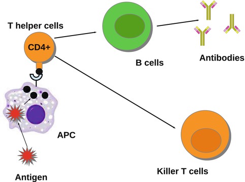
Fig. 14.4
The activation of the immune system by a pathogen
Mathematical models of the interplay of pathogens with the immune system vary from very simple to quite complicated. One of the simplest models was proposed by Gilchrist and Sasaki [65], which includes only the pathogen P(t) and the immune cells B(t):
where r is the pathogen reproduction rate, c is the pathogen clearance rate by the B-cells, and a is the stimulation of B-cell production by the pathogen. This model is very simple, and it can be solved, although an implicit solution is obtained. Problem 14.1 asks you to do that. The model has a set of equilibria with P ∗ = 0 and B ∗ arbitrary:  . Over the long term, the pathogen is always cleared, so the model mimics only acute infection and recovery. This is illustrated in Fig. 14.5. The outcome of the dynamics is sensitive to the initial conditions.
(14.3)
. Over the long term, the pathogen is always cleared, so the model mimics only acute infection and recovery. This is illustrated in Fig. 14.5. The outcome of the dynamics is sensitive to the initial conditions.Fig. 14.5
The activation of the immune system by a pathogen given by system 14.3. Parameters are r = 0. 1, c = 0. 01, a = 0. 0001, P(0) = 10, B(0) = 8
Mohtashemi and Levins [95] considered two other features of the immune system: the spontaneous production of specific cells and their decay. In this case, the model can capture both acute and chronic infection:
where h is the constant production of specific cells, and δ is their clearance rate. The production of B cells is assumed proportional to the pathogen with constant of proportionality k. Model (14.4) has two equilibria: a pathogen-free equilibrium  and a coexistence equilibrium. The coexistence equilibrium is present if and only if the immunological reproduction number
 is greater than one:
  , where
 It can be shown that the coexistence equilibrium is globally stable. More immunological models can be found in the problems section.
(14.4)
and a coexistence equilibrium. The coexistence equilibrium is present if and only if the immunological reproduction number, where14.2.3 Combining Intracellular Pathogen Replication and Immune Response
More complex within-host models combine the intracellular replication of the pathogen and the immune response. The model is based on model (14.1) but includes the killer T-cells, which destroy the infected target cells, and antibodies that help destroy the free pathogen. Both immune responses are stimulated by the pathogen, so they function in competition. The model below was presented in [168]. We denote again by T the target cells, by I the infected target cells, and by V the virus. Killer T-cells are denoted by Z, and antibodies are denoted by A:
Infected target cells are killed at a rate ψ I Z, and pathogen is destroyed at a rate qVA. The killer T-cells’ response is stimulated at a rate aIZ, and the antibodies are stimulated at a rate bVA.
(14.5)
Equilibria of model (14.5) are solutions of the system obtained by setting the right-hand side of system (14.5) to zero. We have a number of solutions of this system. First, we have the infection-free, immune-response-free equilibrium  . Infection develops when the immune reproduction number is greater than one:
 , where
Get Clinical Tree app for offline access

. Infection develops when the immune reproduction number is greater than one:, whereThe system has three more solutions: one in which the killer T-cells are present but the antibody response is not, another in which the antibody response is present but the killer T-cells are not, and finally a third one, in which both immune responses are present. To define the killer T-cells’ immune response, we define a killer T-cell’s invasion number (see Chap. 8)
 If
If  , where
 When the antibody response is present but the killer T-cell response is not, we obtain another equilibrium. The infection, antibody immune response equilibrium exists if the antibody invasion number
  is greater than 1, where
 In this case, we obtain the equilibrium
  , where
 The final equilibrium is an infection, killer T-cells, and antibody response equilibrium with all components present. This equilibrium exists if the killer T-cells’ invasion number in the presence of antibodies
  and the antibody invasion number in the presence of killer T-cells
  are both greater than one. The two invasion numbers are defined as follows:
 We note that
  . The infection, killer T-cells, and antibody response equilibrium
  is given by
The complete analysis of model (14.5) is complex. No oscillations have been found in this model [169].
, where is greater than 1, where, where and the antibody invasion number in the presence of killer T-cells are both greater than one. The two invasion numbers are defined as follows:. The infection, killer T-cells, and antibody response equilibrium is given by(14.6)
14.3 Nested Immuno-Epidemiological Models
Each of the models (14.1), (14.3), (14.4), and (14.5) as well as any other immunological model can be coupled with an appropriate epidemiological model to form a two-scale immuno-epidemiological model. The model that will be formulated and used depends on the disease we want to study as well as the question we would like to address. If we would like to study the impact of medications, we need to use model (14.1), since most medications impact the production of the virus. If we would like to study coevolution, we need to use model (14.3) or model (14.4), since they involve the two variables that evolve in the parasites and the host: the reproduction rate of the parasite r and the immune response of the host a. Coupling model (14.5) with an appropriate epidemiological model may allow us to study both the impact of drugs on the epidemiology of the disease and the coevolution of parasites and hosts. In the next subsection, we will compose a model that will allow us to study the epidemiology of the disease as well as the evolution of the parasite.
14.3.1 Building a Nested Immuno-Epidemiological Model
The first nested immuno-epidemiological model was proposed by Gilchrist and Sasaki [65]. Their goal was to study the coevolution of pathogens and hosts. The idea is simple. The infected individuals in the population are structured by time and time-since-infection i(τ, t), where τ, the time-since-infection, is the independent variable in the immunological model. We take model (14.1) with τ as independent variable. Then T(τ), I(τ), V (τ) are functions of τ. We embed (14.1) into an epidemiological model, say of HIV. We take a simple SI with time-since-infection:
where β(τ) is the transmission rate and m(τ) is the death rate; N is the total population size, and m 0 is the natural death rate:
 The second step in linking the immunological and epidemiological models is to link the epidemiological parameters to the immunological variables. The simplest scenario will be to assume the epidemiological parameters proportional to the viral load. In particular,

The immuno-epidemiological model (14.1)–(14.7) is perhaps one of the simplest models of this type. It has multiple drawbacks:
(14.7)
(14.8)
1.
It assumes that all individuals in the population experience the same within-host dynamics. This problem can be remedied if multiple groups of infected individuals are included in the population.
2.
The immunological model does not experience the growth of the viral load associated with AIDS. This problem can be remedied if an AIDS compartment is included in the epidemiological model:
where A(t) gives the number of people with AIDS. The dependence of the rate of transition to AIDS γ(τ) on the immunological parameters is not clear.
(14.9)
3.
The dependence of β(τ) and m(τ) on the viral load as specified in Eq. (14.8) can be criticized:
The linear dependence of β(τ) is not ideal. In particular, we know that β(τ) = C(τ)q(τ), where C(τ) is the contact rate and q(τ) is the probability of transmission. In HIV, the contact rate either remains constant or decreases with the viral load, as infected individuals become progressively sicker. The probability of transmission increases with the viral load, but it is bounded by 1. Lange and Ferguson [92] found that the dependence of the risk of infection on is best fitted by an S-shaped function. We used the data in [92] to fit the function
  to the data (see Fig. 14.6). The best-fitted parameters were B = 7952. 52 and r = 0. 6. Recalling that
  , we obtain the following function of the viral load:
If the contact rate is assumed constant, the following dependence of β on the viral load is a reasonable approximation of the above function, although [92] suggests a different relationship:
where b is an appropriate constant.
(14.10)
The equation given in (14.8) for m(τ) suggests that given that the viral load is maximal during the acute stage, the maximal death rate is also maximal during the acute stage, which is not the case in HIV. This problem may be remedied by the introduction of an AIDS class.

14.3.2 Analysis of the Immuno-Epidemiological Model
To connect the immunological model to the epidemiology, we compute key epidemiological quantities such as the reproduction number and the prevalence in terms of the immunological quantities. To find the equilibria of the epidemiological model, we consider the system
This system has the disease-free equilibrium  . To compute the endemic equilibrium, we define
 We recall that π(τ) is the probability of survival in the infectious class. We use π(τ) to solve the differential equation: i(τ) = i(0)π(τ). We replace the solution in the third equation in (14.11). After canceling i(0), we obtain the following expression for the fraction of susceptible individuals:
 The fraction of susceptible individuals is less than one. We need the fraction on the right to be less than one. This prompts us to define the following expression as the epidemic basic reproduction number:
(14.11)
. To compute the endemic equilibrium, we define