Screening phase
# of replicates
# concentrations/ sample
Total # of different test samples
Total # of wells
Pilot
2–3
1
103–104
2⋅104
Primary
1
1
105–1.5⋅106
105–1.5⋅106
Confirmation (experiment with replicates)
2–4
1
103–5⋅104
104–2⋅105
Confirmation (experiment with concentration dependent measurements)
1
2–4
103–5⋅104
104–2⋅105
Validation (detailed concentration dependence of response, potency determination)
1–4
8–12
103–5⋅104
104–106
If primary hit rates are very high and cannot be reduced by other means then counter-screens may need to be run in parallel to the primary screen (i.e. one has to run two large screens in parallel!) in order to reduce the number of candidates in the follow phase to a reasonable level and to be able to more quickly focus on the more promising hit compounds. If primary hit rates are manageable in number then such filter experiments (whether counter- or selectivity-screens) can also be run in the confirmation phase. Selectivity measurements are often delayed to the validation screening phase in order to be able to compare sufficient details of the concentration-response characteristics of the compounds which were progressed to this stage on the different targets, and not just have to rely on single-point or only very restricted concentration dependent measurements in the previous phases. Thus, the actual details of the makeup of the screening stages and the progression criteria are highly project dependent and need to be adapted to the specific requirements.
A validation screen, i.e. a detailed measurement of full concentration-response curves with replicate data points and adequately extended concentration range, is then finally done for the confirmed actives, as mentioned, possibly in parallel to selectivity measurements.
The successful identification of interesting small-molecule compounds or other type of samples exhibiting genuine activity on the biological target of interest is dependent on selecting suitable assay setups, but often also on adequate ‘filter’ technologies and measurements, and definitely, as we will see, also on employing the most appropriate statistical methods for data analysis. These also often need to be adapted to the characteristics of the types of experiments and types of responses observed. All these aspects together play an important role for the success of a given HTS project (Sittampalam et al. 2004).
Besides the large full deck screening methods to explore the influence of the of the particular accessible chemical space on the target of interest in a largely unbiased fashion several other more ‘knowledge based’ approaches are also used in a project specific manner: (a) focused screening with smaller sample sets known to be active on particular target classes (Sun et al. 2010), (b) using sets of drug-like structures or structures based on pharmacophore matching and in-silico docking experiments when structural information on the target of interest is available (Davies et al. 2006), (c) iterative screening approaches which use repeated cycles of subset screening and predictive modeling to classify the available remaining sample set into ‘likely active’ and ‘likely inactive’ subsets and including compounds predicted to likely show activity in the next round of screening (Sun et al. 2010), and (d) fragment based screening employing small chemical fragments which may bind weakly to a biological target and then iteratively combining such fragments into larger molecules with potentially higher binding affinities (Murray and Rees 2008).
In some instances the HTS campaign is not executed in a purely sequential fashion where the hit analysis and the confirmation screen is only done after the complete primary run has been finished, but several alternate processes are possible and also being used in practice: Depending on established practices in a given organization or depending on preferences of a particular drug discovery project group one or more intermediate hit analysis steps can be made before the primary screening step has been completed. The two main reasons for such a partitioned campaign are: (a) To get early insight into the compound classes of the hit population and possible partial refocusing of the primary screening runs by sequentially modifying the screening sample set or the sequence of screened plates, a process which is brought to an ‘extreme’ in the previously mentioned iterative screening approach, (b) to get a head start on the preparation of the screening plates for the confirmation run so that it can start immediately after finishing primary screening, without any ‘loss’ of time. There is an obvious advantage in keeping a given configuration of the automated screening equipment, including specifically programmed execution sequences of the robotics and liquid handling equipment, reader configurations and assay reagent reservoirs completely intact for an immediately following screening step. The careful analysis of the primary screening hit candidates, including possible predictive modeling, structure-based chemo-informatics and false-discovery rate analyses can take several days, also depending on assay quality and specificity. The preparation of the newly assembled compound plates for the confirmation screen will also take several days or weeks, depending on the existing compound handling processes, equipment, degree of automation and overall priorities. Thus, interleaving of the mentioned hit finding investigations with the continued actual physical primary screening will allow the completion of a screen in a shorter elapsed time.
RNAi Screening
RNAi ‘gene silencing’ screens employing small ribonucleic acid (RNA) molecules which can interfere with the messenger RNA (mRNA) production in cells and the subsequent expression of gene products and modulation of cellular signaling come in different possible forms. The related experiments and progression steps are varying accordingly. Because of such differences in experimental design aspects and corresponding screening setups also the related data analysis stages and some of the statistical methods will then differ somewhat from the main methods typically used for (plate-based) single-compound small molecule screens. The latter are described in much more depth in the following sections on statistical analysis methods.
Various types of samples are used in RNAi (siRNA, shRNA) screening: (a) non-pooled standard siRNA duplexes and siRNAs with synthetically modified structures, (b) low-complexity pools (3–6 siRNAs with non-overlapping sequences) targeting the same gene, (c) larger pools of structurally similar silencing molecules, for which measurements of the loss of function is assessed through a variety of possible phenotypic readouts made in plate array format in essentially the same way as for small molecule compounds, and also—very different—(d) using large scale pools of shRNA molecules where an entire library is delivered to a single population of cells and identification of the ‘interesting’ molecules is based on a selection process.
RNAi molecule structure (sequence) is essentially known when using approaches (a) to (c) and, thus, the coding sequence of the gene target (or targets) responsible for a certain phenotypic response change can be inferred in a relatively straightforward way (Echeverri and Perrimon 2006; Sharma and Rao 2009). RNAi hit finding progresses then in similar way as for compound based screening: An initial primary screening run with singles or pools of related RNAi molecule samples, followed by a confirmation screen using (at least 3) replicates of single or pooled samples, and if possible also the individual single constituents of the initial pools. In both stages of screening statistical scoring models to rank distinct RNAi molecules targeting the same gene can be employed when using pools and replicates of related RNAi samples (redundant siRNA activity analysis, RSA, König et al. 2007), thus minimizing the influence of strong off-target activities on the hit-selection process. In any case candidate genes which cannot be confirmed with more than one distinct silencing molecule will be eliminated from further investigation (false positives). Birmingham et al. (2009) give an overview over statistical methods used for RNAi screening analysis. A final set of validation experiments will be based on assays measuring the sought phenotypic effect and other secondary assays to verify the effect on the biological process of interest on one hand, and a direct parallel observation of the target gene silencing by DNA quantitation, e.g. by using PCR (polymerase chain reaction) amplification techniques). siRNA samples and libraries are available for individual or small sets of target genes and can also be produced for large ‘genome scale’ screens targeting typically between 20,000 and 30,000 genes.
When using a large-scale pooled screening approach, as in d) above, the selection of the molecules of interest and identification of the related RNA sequences progresses in a very different fashion: In some instances the first step necessary is to sort and collect the cells which exhibit the relevant phenotypic effect (e.g. the changed expression of a protein). This can for example be done by fluorescence activated cell sorting (FACS), a well-established flow-cytometric technology. DNA is extracted from the collected cells and enrichment or depletion of shRNA related sequences is quantified by PCR amplification and microarray analysis (Ngo et al. 2006). Identification of genes which are associated with changed expression levels using ‘barcoded’ sets of shRNAs which are cultured in cells both under neutral reference conditions and test conditions where an effect-inducing agent, e.g. a known pathway activating molecule is added (Brummelkamp et al. 2006) can also be done through PCR quantification, or alternatively through massive parallel sequencing (Sims et al. 2011) and comparison of the results of samples cultured under different conditions. These are completely ‘non-plate based’ screening methods and will not be further detailed here.
5.2 Statistical Methods in HTS Data Analysis
5.2.1 General Aspects
In the next sections we will look at the typical process steps of preparing and running a complete HTS campaign, and we will see that statistical considerations play and important role in essentially all of them because optimal use of resources and optimal use of information from the experimental data are key for a successful overall process. In the subsequent sections of this chapter we will not touch on all of these statistical analysis aspects with the same depth and breadth, not least because some of these topics are actually treated in more detail elsewhere in this book, or because they are not very specific to HTS data analysis. We will instead concentrate more on the topics which are more directly related to plate-based high-throughput bioassay experiments and related efficient large scale screening data analysis.
5.2.2 Basic Bioassay Design and Validation
Given a particular relevant biological target the scientists will need to select the assay method, detection technology and the biochemical parameters. This is sometimes done independently from HTS groups, or even outside the particular organization. Primarily the sensitivity (ability to detect and accurately distinguish and rank order the potency of active samples over a wide range of potencies, e.g. based on measurements with available reference compounds) and reproducibility questions need to be investigated in this stage. Aspects of specificity in terms of the potential of a particular assay design and readout technology to produce signals from compounds acting through unwanted mechanisms as compared to the pharmacologically relevant mechanism also need to be assessed.
The exploration and optimization of assay conditions is usually done in various iterations with different series of experiments employing (fractional) factorial design, replication and response surface optimization methods to determine robust response regions. The potentially large series of assay parameters (selection of reagents, concentrations, pH, times of addition, reaction time courses, incubation times, cell numbers, etc.) need to be investigated at multiple levels in order to be able to detect possible nonlinearities in the responses (Macarron and Hertzberg 2011). The practical experimentation involving the exploration of many experimental factors and including replication often already takes advantage of the existing screening automation and laboratory robotics setups to control the various liquid handling steps, which otherwise would be rather cumbersome and error-prone when performed manually (Taylor et al. 2000). Standard methods for the analysis of designed experiments are used to optimize dynamic range and stability of the assay readout while maintaining sensitivity (Box et al. 1978; Dean and Lewis 2006). Most often the signal-to-noise ratio SNR, signal window SW and Z′-factor are used as optimization criteria. See the section on assay quality measures and Table 5.2 below for the definition of these quantities.
Table 5.2
Selected assay quality metrics
Quality control measure | Estimation expression | Comments | |
|---|---|---|---|
a | Coefficient of Variation for Controls and References, CV |  | Simple statistic giving rough indication of signal variability, without consideration of actual range of obtainable responses |
b | High/Low Ratio, HLR Signal/Background Ratio, SBR |  , ,  | HLR and SBR quantify the ratio of the maximal to minimal response values but without considering the variability of the signals |
c | Signal/Noise Ratio, SNR |  | ‘Dynamic range’ of signal in relation to standard deviation of neutral controls. Variation of positive controls not taken into account |
d | Signal Window Coefficient, SW |  | Akin to SNR, but only considering signal range ‘outside’ of 3s limits of the controls, i.e. the ‘usable’ signal window to quantify responses differing from the controls (Sittampalam et al. 1997) |
e | Z′-factor RZ′-factor (robust) Assay Window Coefficient |  | Use of mean  and standard deviation s x for Z′ or median and standard deviation s x for Z′ or median  and mad estimators and mad estimators  for RZ′, respectively. Ratio of ‘usable’ signal window size outside of 3s limits in relation to the full signal range (relative signal window size between controls) (Zhang et al. 1999) for RZ′, respectively. Ratio of ‘usable’ signal window size outside of 3s limits in relation to the full signal range (relative signal window size between controls) (Zhang et al. 1999) |
f | V-factor Conceptually related to Z′-factor, but also considering the variation of a set of intermediate response values, not just the variation at the response range limits |  | |
g | SSMD, strictly standardized mean difference |  | SSMD expressions for unequal variance and unequal sample sizes can be found in Zhang et al. (2007). SSMD estimates tends to be closer to population values than the equivalent t-statistics. In practice SSMD statistics are predominantly used to assess the significance of effect sizes in RNAi screening, see Zhang (2008, 2011a, b) |


Instead of mean  and standard deviation s estimators the median
  and mad
  can be used as robust plug-in replacements
and standard deviation s estimators the median and mad can be used as robust plug-in replacements5.2.3 Assay Adaptation to HTS Requirements and Pilot Screening
The adaptation of assay parameters and plate designs with respect to the positioning and numbers of control samples, types of plates, plate densities and thus, liquid volumes in the individual plate wells, to fulfill possible constraints of the automated HTS robotics systems needs to follow, if this was not considered in the initial assay design, e.g. when the original bioassay was designed independently of the consideration to run it as a HTS. The initially selected measurement technology often has an influence on the obtainable screening throughput. If these design steps were not done in initial collaboration with the HTS groups, then some of the assays parameters may have to be further changed and optimized with respect to relevant assay readout quality measures (see Table 5.2) for the assay to be able to run under screening conditions. Again, experimental design techniques will be employed, albeit with a now much reduced set of factors. These assay quality metrics are all based on the average response levels  of different types of controls, corresponding to readout for an inactive probe (N, neutral control) or the readout for a ‘fully active’ probe (P, positive control) and the respective estimates of their variability (standard deviation) s.
of different types of controls, corresponding to readout for an inactive probe (N, neutral control) or the readout for a ‘fully active’ probe (P, positive control) and the respective estimates of their variability (standard deviation) s.The quality control estimators in Table 5.2 are shown as being based on the mean  and standard deviation s, but in practice the corresponding outlier resistant ‘plug-in’ equivalents using the median
  and median absolute deviation (mad)
  estimators are often used, where
  includes the factor 1.4826 to ensure consistency with s, so that
  if
if  ) (Rousseeuw and Croux 1993).
and standard deviation s, but in practice the corresponding outlier resistant ‘plug-in’ equivalents using the median and median absolute deviation (mad) estimators are often used, where includes the factor 1.4826 to ensure consistency with s, so that if ) (Rousseeuw and Croux 1993).The quality measures which incorporate information on variability of the controls often much more useful than simple ratios of average values because probability based decision making in the later hit selection process needs to take into account the distributions of the activity values. In order to gain a quick overview and also see aspects of the distribution of the measured values (e.g. presence of outliers, skewness) which are not represented and detected by the simple statistical summary values the data should always be visualized using e.g. categorized scatterplots, boxplots, strip plots and normal quantile-quantile plots.
Possible modifications of the original assay design may entail gaining higher stability of response values over longer time scales or in smaller volumes to be able to run larger batches of plates, shortening some biochemical reaction or incubation phases to gain higher throughput, or to have smaller influence of temperature variations on responses, etc. Such modifications may sometimes even have to be done at the cost of reduced readout response levels. As long as the assay quality as measured by a suitable metric stays above the acceptance criteria defined by the project group such ‘compromises’ can usually be done without large consequences for the scientific objectives of the HTS project.
Besides the optimization of the assay signal range and signal stability an important part of the quality determination and validation in the assay adaptation phase is the initial determination of assay reproducibility for samples with varying degrees of activity using correlation- and analysis of agreement measures, as well providing rough estimates on expected false positive and false negative rates which are based on the evaluation of single point %-activity data at the planned screening concentration and the determination of the corresponding concentration-response data as an activity reference for the complete standard ‘pilot screening library’ of diverse compounds with known mechanisms of action and a wide range of biological and physicochemical properties for use in all HTS assays in the pilot screening phase (Coma et al. 2009a, b). See Table 5.3 for an overview of typical analyses performed in this phase.
Table 5.3
Quality metrics and methods in assay adaptation and pilot screening phase
Type of analysis, metric | Methods, tools | Comments | |
|---|---|---|---|
a | Correlation analysis | Pearson correlation coefficient ρ (n = 2), Spearman rank correlation (n = 2), intraclass correlation coefficient ICC (n > 2) | |
b | Analysis of agreement | Bland–Altman plot, scale-location plots:  or or  , where s is the standard deviation and Δ is the range of data at a particular , where s is the standard deviation and Δ is the range of data at a particular  value value | |
c | Normality, deviation from normality | Normal probability plot, Kolmogorov–Smirnov Test, Anderson–Darling Test | Comparison of control and reference sample distributions with normal distributions (Wu and Liu 2008) |
d | Initial estimate of expected false positive (FP) and false negative (FN) rates | Comparison of primary screening results with results of concentration response experiments | |
e | MSR, minimum significant ratio (smallest potency ratio between compounds which is statistically significant at level α, usually α = 0.05) | ![$$ \begin{aligned} {}\\[-12pt] {10}^{Z_{\alpha /2}\sqrt{2}\hat{s}}\end{aligned} $$](/wp-content/uploads/2016/07/A330233_1_En_5_Chapter_IEq28.gif) where  is the sample standard deviation of a set of independent repeated log10(IC 50) potency determinations and Z α/2 the standard normal distribution quantile is the sample standard deviation of a set of independent repeated log10(IC 50) potency determinations and Z α/2 the standard normal distribution quantile |
These investigations with the standard pilot screening library will sometimes also allow one to gain early information on possible selectivity (to what extent are compounds acting at the target vs. other targets of the same family) and specificity (is the compound acting through the expected mechanism or through an unwanted one) of the assay for an already broader class of samples available in the pilot screening library than are usually investigated in the initial bioassay design.
While the detailed evaluation of factors and response optimization using experimental design approaches with replicated data are feasible (and necessary) at the assay development and adaptation stages, this is no longer possible in the actual large primary HTS runs. They will usually need to be executed with n = 1 simply because of the large scale of these experiments with respect to reagent consumption, overall cost and time considerations. Because of this bulk- and batch execution nature of the set of measurements collected over many days or weeks it is not possible to control all the factors affecting the assay response. Given these practical experimental (and resource) restrictions, the observed random and systematic variations of the measured responses need to be accommodated and accounted for in the data analysis steps in order to extract the highest quality activity- and activity-rank order information possible. The use of optimal data normalization and hit selection approaches are key in this respect.
5.2.4 Assay Readouts, Raw and Initial Derived Values
Raw readouts from plate readers are generated in some instrument-specific units (often on an ‘arbitrary’ scale) which can be directly used for data quality and activity assessment, but in other assay setups there may be a need for an initial data transformation step. This can be needed when performing time- or temperature-dependent measurements which need a regression analysis step to deliver derived readouts in meaningful and interpretable physical units (assay readout endpoints), e.g. using inverse estimation on data of a calibration curve, determining kinetic parameters of a time-course measurement or protein melting transition temperatures in a thermal shift assay, or extracting the key time course signal characteristics in a kinetic fluorescence intensity measurement. Sometimes such derived information can be obtained directly from the instrument software as an alternate or additional ‘readout’, but when developing new assays and measurement methods it is sometimes necessary to be able to add different, more sophisticated or more robust types of analyses as ad-hoc data preprocessing steps. It is a definite advantage if a standard software framework is available where such additional analysis steps and related methods can be easily explored, developed and readily plugged into the automated assay data processing path, e.g. by using R scripts (R Development Core Team 2013) in the Pipeline Pilot® (http://accelrys.com/products/pipeline-pilot/), Knime (https://www.knime.org/) or similar analytics platform included upstream of an organization’s standard screening data processing system, where data thus transformed can then easily be processed using the available standard HTS data analysis methods in the same way as any other type of screening reader output.
Assay and readout technologies have gone through many changes and advancements in the past years. Whereas initially in HTS the measurement of only one or very few (2–3) readout parameters per well (e.g. fluorescence intensities at two different wavelengths) was customary—and still is for many practical applications—the advent of automated microscopy and cellular imaging coupled with automated image analysis (image based High Content Analysis or Screening, HCA, HCS) which can detect changes in the morphology of cells or of separately labeled cell compartments (nucleus, membrane, organelles, etc.), thus resulting in a large number of parameters for a given well or even for each individual cell, has led to the need for the exploration and evaluation of suitable multivariate statistical data analysis methods (Hill et al. 2007). Intensities, textures, morphological and other parameters from the segmented images are captured at several different wavelengths and corresponding feature vectors are associated with each identified object or well (Abraham et al. 2004; Carpenter 2007; Duerr et al. 2007; Nichols 2007). Cell level analysis enables the analysis of the various cell-cycles and the separation of the effects of the probes on cells in a particular state (Loo et al. 2007; Singh et al. 2014). Besides the now quite broadly used image based HCS approaches there are several other assay technologies which produce multivariate readouts of high dimensions, Cytof (Qiu et al. 2011), Luminex gene expression profiling (Wunderlich et al. 2011), RPA (van Oostrum et al. 2009), laser cytometry (Perlman et al. 2004 ), and others, with medium throughput . For most of these technologies the most suitable optimal data analysis methods are still being explored. Questions of normalization, correction of systematic errors, discrimination and classification are under active investigation in many labs (Reisen et al. 2013; Kümmel et al. 2012; Abraham et al. 2014; Singh et al. 2014; Smith and Horvath 2014; Haney 2014). It is clear that all these different types of assay technologies can benefit from a common informatics infrastructure for large scale multivariate data analysis, which includes a large set of dimension reduction, feature selection, clustering, classification and other statistical data analysis methods, as well as a standardized informatics systems for data storage and metadata handling, coupled to high performance computing resources (compute clusters) and large volume file stores and databases (Millard et al. 2011).
The high numbers of readout parameters (300–600) (Yin et al. 2008; Reisen et al. 2013) which must be simultaneously analyzed and the much higher data volumes which need to be processed introduce new aspects into high-throughput screening data analysis which are usually not covered by the available features in the established standard screening informatics systems (Heyse 2002; Gunter et al. 2003; Kevorkov and Makarenkov 2005; Gubler 2006; Boutros et al. 2006; Zhang and Zhang 2013). This makes these data much more challenging to analyze from the point of view of methodology, complexity of assay signals and the sheer amounts of data. But it is clear that these types of screening technologies and efficient methods to analyze the large data volumes will become even more important and widespread in future. While one can say that the analysis methods for standard HTS data have been largely settled—at least from the point of view of the main recommended data processing and quality assurance steps as outlined in this chapter—this is definitely not yet the case for the high dimensional multivariate screening data analysis, especially when going to the single cell level. Note that the screening literature occasionally refers to multi–parametric analysis in this context. Systematic investigations on advantages and disadvantages of particular methods and the preferred approaches for determining assay and screening quality metrics, correction of systematic response errors, classification of actives, etc. with such types of data are ongoing and are naturally more complex than for the cases where just a few readout parameters can be processed in a largely independent manner up to the point where the final values need to be correlated to each other (Kümmel et al. 2012).
5.2.5 Assay Quality Measures
The overall error which accumulates over the many different chemical, biological and instrumental processing steps to obtain the final readout in a screening assay needs to be kept as small as possible so that there is high confidence in the set of compounds identified as active in a screening campaign. The assay quality metrics to measure and monitor this error are based on simple location and scale estimates derived from raw readout data from the different types of wells on a microtiter plate (zero-effect and full inhibition of full activation controls for normalization of the data, reference controls exhibiting responses in the middle of the expected response range, background wells, and test sample wells). Different quality indicators have been proposed to measure the degree of separability between positive and zero-effect (neutral) assay controls: Signal to background ratio or high-low ratio, coefficient of variation, signal to noise ratio, Z– and Z′-factor (not to be confused with a Z-score) (Zhang et al. 1999), strictly standardized mean difference (SSMD) (Zhang et al. 2007) and others are in routine use to optimize and measure assay response quality (see Table 5.2).
The Z′-factor has become an accepted and widely used quality metric to assess the discriminatory power of a screening assay. It is a relative measure and quantifies the ‘usable window’ for responses between the upper and lower controls outside of their respective 3s limits. Z′ can be between  (if the control averages which define the response limits are identical), 0 when the two 3s limits ‘touch’ each other, and 1 if the standard deviation of the controls becomes vanishingly small. Z′ is an empirical point measure and the derivation of its large sample interval estimator was only recently published (Majumdar and Stock 2011). The sampling uncertainty of Z′ should be considered when setting acceptance thresholds, especially for lower density plates with small numbers of control wells. Small sample intervals can be estimated by bootstrap resampling (Iversen et al. 2006). Other quality indicators than those listed were proposed and described in the literature (e.g. assay variability ratio, signal window and others), but are not so widely used in standard practice because they are related to the Z′-factor and don’t represent independent information (Sui and Wu 2007; Iversen et al. 2006). The V-factor is a generalization of the Z′-factor to multiple response values between
  and
and  (Ravkin 2004).
(if the control averages which define the response limits are identical), 0 when the two 3s limits ‘touch’ each other, and 1 if the standard deviation of the controls becomes vanishingly small. Z′ is an empirical point measure and the derivation of its large sample interval estimator was only recently published (Majumdar and Stock 2011). The sampling uncertainty of Z′ should be considered when setting acceptance thresholds, especially for lower density plates with small numbers of control wells. Small sample intervals can be estimated by bootstrap resampling (Iversen et al. 2006). Other quality indicators than those listed were proposed and described in the literature (e.g. assay variability ratio, signal window and others), but are not so widely used in standard practice because they are related to the Z′-factor and don’t represent independent information (Sui and Wu 2007; Iversen et al. 2006). The V-factor is a generalization of the Z′-factor to multiple response values between and (Ravkin 2004).Some screening quality problems can occur for actual sample wells which are not captured by control well data and the measures listed in Table 5.2, e.g. higher variability for sample wells than for control wells, additional liquid handling errors due to additional process steps for sample pipetting, non-uniform responses across the plates, etc. Such effects and tools for their diagnosis are described in more detail further below in the screening data quality and process monitoring section.
In Fig. 5.1 we show an example of the behavior of the High/Low control ratio (HLR) and the Z′ factor for a set of 692 1536-well plates from a biochemical screen exhibiting several peculiarities: (a) clear batch boundary effects in the ratio of the HLR values for batch sizes varying between 80 and 200 plates, (b) ‘smooth’ time dependence of the HLR (fluorescence intensity) ratio due to the use of continuous assay product formation reaction and related detection method, (c) no ‘strongly visible’ influence of the varying HLR on the Z′-factor, i.e. a negligible influence of the varying HLR on the relative ‘assay window’, (d) an interleaved staggering pattern of HLR which is due to the use of a robotic system with two separate processing lanes with different liquid handling and reader instruments. This latter aspect may be important to take into account when analyzing the data because any systematic response errors, if they occur at a detectable and significant level, are likely to be different between the two subsets of plates, hence a partially separate analysis may need to be envisaged. We also see that for assays of this nature setting a tight range limit on HLR will not make sense; only a lower threshold could be useful as a potential measurement failure criterion.
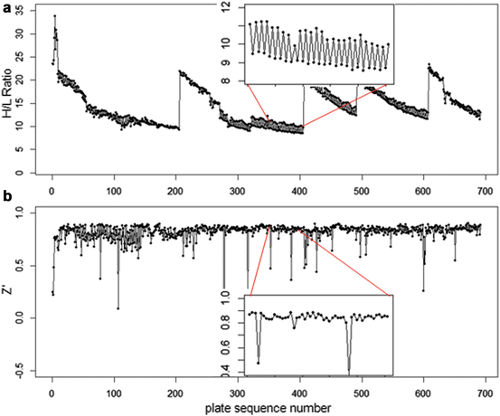
Fig. 5.1
(a) Screening quality control metrics: High/Low ratio HLR for complete screening run showing batch start and end effects, signal changes over time and alternating robot lane staggering effects (inset). (b) Z′-factor (assay window coefficient) for the same plate set with occasional low values for this metric, indicating larger variance of control values for individual plates, but generally negligible influence of robot lane alternation on assay data quality (inset, saw tooth pattern barely visible)
5.2.6 Screening Data Quality and Process Monitoring
Automated screening is executed in largely unattended mode and suitable procedures to ensure that relevant quality measures are staying within adequate acceptance limits need to be set up. Some aspects of statistical process control (SPC) methodology (Shewhart 1931; Oakland 2002) can directly be transferred to HTS as an ‘industrial’ data production process (Coma et al. 2009b; Shun et al. 2011).
Data quality monitoring of larger screens using suitably selected assay quality measures mentioned above and preferably also for some of the additional screening quality measures listed below in Table 5.4, can be done online with special software tools which analyze the data in an automated way directly after the readout is available from the detection instruments (Coma et al. 2009b), or at least very soon after completing the running of a plate batch with the standard data analysis tools which are in use, so that losses, potential waste and the need for unnecessarily repetitions of larger sets of experiments are minimized. As in every large scale process the potential material and time-losses and the related financial aspects cannot be neglected and both plate level and overall batch level quality must be maintained to ensure a meaningful completion of a screening campaign.
Table 5.4
Screening quality metrics
Metric | Estimation expression | Comments | |
|---|---|---|---|
a | Z-factor RZ-factor (robust) Screening Window Coefficient |  | Mean, standard deviation or median, mad use in the same way as for Z′/RZ′ factor (Zhang et al. 1999) |
b | Maximum, minimum, or range of systematic error  on plate p on plate p |  , ,  , , | H. Gubler, 2014, unpublished work |
c | VEP, Fraction of response variance ‘explained’ by the estimated systematic error components (pattern) on plate p |  | Coma et al. (2009b) |
d | Moran’s I, spatial autocorrelation coefficient |  with neighbor weights w ij (e.g. w ij = 1 if i and j are neighbor wells within a given neighborhood distance δ, e.g. δ = 2, sharing boundaries and corner points, and w ij = 0 otherwise, and also  ). Also distance based weights ). Also distance based weights  can be used can be used | Use for statistical test of null hypothesis that no significant spatial correlation is present on a plate, i.e. no systematic location dependent sample response deviation from the average null-effect response exists (Moran 1950; Murie et al. 2013) Other spatial autocorrelation coefficients can also be used for this test, e.g. Geary’s C ratio (Geary 1954) |
These measures are focused on sample-well area of plates
Instead of mean  and standard deviation s estimators the median
  and mad
  are often used as robust plug-in replacements. In order to roughly determine systematic error estimates
  in the initial HTS monitoring stage a model which is very quickly calculated can be chosen (e.g. spatial polish, polynomial or principal pattern models, see Table 5.6). For the final analysis of the screening production runs the most suitable error modeling method for the determination of the systematic plate effects will be used and the screening quality measures before and after correcting the data for the systematic errors can be compared
and standard deviation s estimators the median and mad are often used as robust plug-in replacements. In order to roughly determine systematic error estimates in the initial HTS monitoring stage a model which is very quickly calculated can be chosen (e.g. spatial polish, polynomial or principal pattern models, see Table 5.6). For the final analysis of the screening production runs the most suitable error modeling method for the determination of the systematic plate effects will be used and the screening quality measures before and after correcting the data for the systematic errors can be comparedSystematic response errors in the data due to uncontrolled (and uncontrollable) factors will most likely also affect some of the general and easily calculated quality measures shown in Table 5.4, and they can thus be indirect indicators of potential problems in the screening or robotic automation setup. When using the standard HTS data analysis software tools to signal the presence of systematic response errors or a general degradation of the readout quality, then the broad series of available diagnostic tools can efficiently flag and ‘annotate’ any such plate for further detailed inspection and assessment by the scientists. This step can also be used to automatically categorize them for inclusion or exclusion in a subsequent response correction step.
A note on indexing in mathematical expressions: In order to simplify notation as far as possible and to avoid overloading the quoted mathematical expressions we will use capital index letters to indicate a particular subset of measured values (e.g. P and N as previously mentioned, C compound samples), and we will use single array indexing of measured or calculated values of particular wells i whenever possible. In those situations where the exact row and column location of the well in the two-dimensional grid is important we will use double array indexing ij. The explicit identification of the subset of values on plate p is almost always required, so this index will appear often.
These additional metrics are relying on data from the sample areas of the plates and will naturally provide additional important insight into the screening performance as compared to the control sample based metrics listed in Table 5.2. As for the previously mentioned control sample based assay quality metrics it is even more important to visualize such additional key screening data quality metrics which are based on the (compound) sample wells in order to get a quick detailed overview on the behavior of the response data on single plates, as well as its variation over time to obtain indications of data quality deteriorations due to instrumental (e.g. liquid handling failures), environmental (e.g. evaporation effects, temperature variations) and biochemical (e.g. reagent aging) factors, or due to experimental batch effects, e.g. when using different reagent or cell batches. Direct displays of the plate data and visualizations of the various assay quality summaries as a function of measurement time or sequence will immediately reveal potentially problematic data and suitable threshold settings can trigger automatic alerts when quality control metrics are calculated online.
Some of the listed screening quality metrics are based on direct estimation of systematic plate and well-location specific experimental response errors S ijp , or are indicators for the presence of spatial autocorrelation due to localized ‘background response’ distortions, e.g. Moran’s I coefficient which also allows the derivation of an associated p-value for the ‘no autocorrelation’ null hypothesis (Moran 1950). Similar visualizations as for the HLR and Z′-factor shown in Fig. 5.1 can also be generated for the listed screening quality metrics, like the Z-factor (screening window), Moran coefficient I, or the VEP measure.
In Fig. 5.2 we show examples of useful data displays for response visualizations of individual plates. In this case both the heatmap and the separate platewise scatterplot of all data, or boxplots of summary row- and column effects of a 384-well plate clearly show previously mentioned systematic deviations of the normalized response values which will need to be analyzed further. In the section on correction of systematic errors further below we also show an illustration of the behavior of the Moran coefficient in presence of systematic response errors, and after their removal (Fig. 5.6).
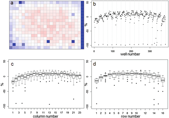
Fig. 5.2
(a) Example plate data heatmap showing visibly lower signal in border areas due to evaporation effects. (b) Scatterplot of normalized response values of all individual wells with grid lines separating different plate rows. (c) Boxplot of column summaries, and (d) Boxplot of row summaries, all showing location dependent response differences across the plate and offsets of row- and column medians from 0
It is also recommended to regularly intersperse the screening plate batches with sets of quality control plates without compounds (providing a control of liquid handling performance) and plates containing only inhibitor or activator controls and, if relevant, further reference compound samples exhibiting intermediate activity to provide additional data on assay sensitivity. ‘QC plates’ without compounds or other types of samples (just containing assay reagents and solvents) are also very helpful for use in correcting the responses on the compound plates in cases where it is not possible to reliably estimate the systematics errors from an individual plate or a set of sample plates themselves. This is e.g. the case for plates with large numbers of active samples and very high ‘hit rates’ where it is not possible to reliably determine the effective ‘null’ or ‘background’ response, as well as for other cases where a large number of wells on a plate will exhibit nonzero activity, especially also all concentration- response experiments with the previously selected active samples from the primary screens. For these situations we have two possibilities to detect and correct response values: (a) Using the mentioned QC control plates (Murie et al. 2014), and (b) using plate designs with ‘uniform’ or ‘uniform random’ placement of neutral control wells across the whole plate, instead of placing the controls in a particular column or row close to the plate edges (Zhang 2008), as is often done in practice. Such an arrangement of control well locations will allow the estimation of systematic spatial response deviations with the methods which only rely on a small number of free parameters to capture the main characteristics and magnitude of the background response errors, as e.g. polynomial response models.
5.2.7 Integration of Diagnostic Information from Automated Equipment
Modern liquid handlers (e.g. acoustic dispensers) often have the capability to deliver success/failure information on the liquid transfer for each processed well and this information can be automatically joined with the reader data through plate barcode and well matching procedures, and then considered for automated valid/invalid flagging of the result data, provided suitable data management processes and systems are available. Also other types of equipment may be equally able to signal failures or performance deterioration at the plate or well level which then can also be correlated with reader data and be integrated in suitable alerting and flagging mechanisms for consideration during data analysis.
5.2.8 Plate Data Normalization
Uncontrolled experimental factors will influence the raw assay readouts on each individual plate. This can be likened to the existence of multiplicative and possibly also additive systematic errors between individual plates p which can be represented by the measurement model 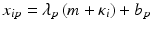 , where x ip is the measured raw value in well i on plate p , m is the ‘intrinsic’ null-effect response value of the assay, κ i is a sample (compound) effect, with κ i = 0 if inactive, and λ p and b p are plate-, instrument- and concentration dependent gain factors and offsets, respectively. x ip can then also equivalently be represented as
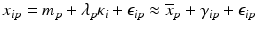
when also including an error term 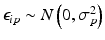 and setting
 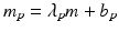 ,
,  . We make
  explicitly depend on plate index p because this often corresponds to experimental reality, especially between different plate batches. Reagent aging and evaporation as well as time shifts in some process steps will usually lead to smooth trends in plate averages within batches, whereas e.g. the effect of cells plated at very different times may show up as a more discrete batch effect of responses. Plate-level normalization procedures use the response values of specific wells to bring the response values into a standardized numerical range which can be easily interpreted by scientists, usually a 0–100 % scale with respect to the no-effect and the ‘maximal’ effect obtainable with the given assay parameters. In this particular context ‘plate normalization’ is simply understood to adjust the average responses between the different plates: Control based normalization via specifically selected control wells, sample based normalization via the ensemble of all sample wells if the number of active wells is ‘small enough’. The use of robust estimation procedures with high breakdown limits is critical for successful sample based normalization because of the likely presence of ‘outliers’, i.e. active compounds with larger response deviations in usually one and sometimes both possible response directions.
, where x ip is the measured raw value in well i on plate p , m is the ‘intrinsic’ null-effect response value of the assay, κ i is a sample (compound) effect, with κ i = 0 if inactive, and λ p and b p are plate-, instrument- and concentration dependent gain factors and offsets, respectively. x ip can then also equivalently be represented as(5.1)
and setting , . We make explicitly depend on plate index p because this often corresponds to experimental reality, especially between different plate batches. Reagent aging and evaporation as well as time shifts in some process steps will usually lead to smooth trends in plate averages within batches, whereas e.g. the effect of cells plated at very different times may show up as a more discrete batch effect of responses. Plate-level normalization procedures use the response values of specific wells to bring the response values into a standardized numerical range which can be easily interpreted by scientists, usually a 0–100 % scale with respect to the no-effect and the ‘maximal’ effect obtainable with the given assay parameters. In this particular context ‘plate normalization’ is simply understood to adjust the average responses between the different plates: Control based normalization via specifically selected control wells, sample based normalization via the ensemble of all sample wells if the number of active wells is ‘small enough’. The use of robust estimation procedures with high breakdown limits is critical for successful sample based normalization because of the likely presence of ‘outliers’, i.e. active compounds with larger response deviations in usually one and sometimes both possible response directions.Normalization of Compound Screening Data
In the experiment- and plate design for small molecule compound screening one usually has two types of controls to calibrate and normalize the readout signals to a 0–100 % effect scale: A set of wells (neutral or negative controls) corresponding to the zero effect level (i.e. no compound effect) and a set of wells (positive controls) corresponding to the assay’s signal level for the maximal inhibitory effect, or for activation- or agonist assays, corresponding to the signal level of an effect-inducing reference compound. In the latter case the normalized %-scale has to be understood to be relative to the chosen reference which will vary between different reference compounds, if multiple are known and available, and hence has a ‘less absolute’ meaning compared to inhibition assays whose response scale is naturally bounded by the signal level corresponding to the complete absence of the measured biological effect. In some cases an effect-inducing reference agonist agent may not be known and then the normalization has to be done with respect to neutral controls only, i.e. using Fold- or any of the Z– or R-score normalization variants shown in Table 5.5.
Table 5.5
Data normalization and score calculations
Normalization or scoring measure | Estimation expression | Comment | |
|---|---|---|---|
a | Percent of Control | 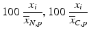 | Compensates for plate to plate differences in N = neutral control/negative control average (no compound effect) or C = sample average |
b | (Normalized) Percent Inhibition (NPI) or Normalized Percent Activation/Percent Activity (NPA) with appropriately chosen neutral N and positive P controls | 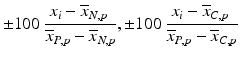 | N = neutral control/negative control (=no compound effect), P = positive control (=full inhibition or full activation control) Can also be based on sample (compound) average  of each plate instead of neutral control average of each plate instead of neutral control average  |
c | Percent Change | 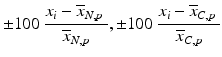 | (see comment for row b) |
d | Fold (control based, sample based) |  | Based on neutral control average  or sample average or sample average  of each plate of each plate |
e | Z-score, using mean and standard deviation estimators for  and s x , respectively and s x , respectively |  | Compensates for plate to plate differences in average value and variance s x can be determined from negative controls N or from samples C: s x = s N or s x = s S |
f | R-score, similar to Z-score, but using median and mad estimators  and and  , respectively , respectively |  | Often preferred over Z-scores because of relatively frequent presence of outliers and/or asymmetries in the distributions |
g | One-sided Z– or R-scores. Scoring only for samples which exhibit an effect in the desired direction | Separate Z– or R-scores for  , or , or  with calculation of s x for corresponding subset only with calculation of s x for corresponding subset only | Compensates for plate to plate differences in average and in variance for asymmetric distributions |
h | Generalized R-score calculation of platewise or batchwise corrected response values. Scoring after elimination of estimated systematic error S at each plate/well location. |  where < div class='tao-gold-member'>
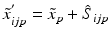 is the ‘true’ null-effect reference response which is corrected for the estimated spatial and temporal systematic errors is the ‘true’ null-effect reference response which is corrected for the estimated spatial and temporal systematic errors  , and the scale , and the scale  is calculated from the data after this location-dependent data re-centering step is calculated from the data after this location-dependent data re-centering stepOnly gold members can continue reading. Log In or Register to continue
Stay updated, free articles. Join our Telegram channel
Full access? Get Clinical Tree
 Get Clinical Tree app for offline access

|