–![$$\,d]$$](/wp-content/uploads/2016/10/A324942_1_En_2_Chapter_IEq2.gif) -damage formulation, where only the anisotropic elastic part is assumed to damage. The resulting coupled, highly non-linear system of equations is symmetric and can conveniently be solved by standard incremental-iterative Newton-Raphson schemes or arc-length-based solution methods without any need for advanced and computationally expensive solution methods such as a global active-set-search as applied by Liebe et al. [11]. Furthermore, the approach proves to be robust, even at high levels of degradation, and allows to incorporate any suitable scalar-valued damage formulation.
-damage formulation, where only the anisotropic elastic part is assumed to damage. The resulting coupled, highly non-linear system of equations is symmetric and can conveniently be solved by standard incremental-iterative Newton-Raphson schemes or arc-length-based solution methods without any need for advanced and computationally expensive solution methods such as a global active-set-search as applied by Liebe et al. [11]. Furthermore, the approach proves to be robust, even at high levels of degradation, and allows to incorporate any suitable scalar-valued damage formulation.
Apart from the highly nonlinear elastic response of soft biological tissues, it is well-known that the structural design of arteries is characterised by a fibre-reinforced multi-layered composite subjected to pronounced residual stresses. The complex interaction of material properties with these residual stress effects and the geometry guarantees the optimal support under different blood pressures within the vessel. As a further key aspect of this contribution, we therefore incorporate residual stresses by means of a multiplicative composition of the deformation gradient.
This article is structured as follows: In Sect. 2, we summarise relevant kinematic relations for the geometrically non-linear case and the balance equations of the coupled boundary value problem in weak form. In Sect. 3, we specify the underlying constitutive equations, containing the isotropic and anisotropic non-linear elastic and gradient-enhanced free energies, as well as the continuum damage formulation. In Sect. 4, we discretise the governing weak forms by means of the finite element method resulting in a coupled non-linear system of equations. Last, in Sect. 6, we apply the model to illustrative three-dimensional inhomogeneous deformation problems. In order to show the capabilities of the approach with regard to biomechanics-related problems, we study a force-driven finite element example by means of an anisotropic artery-like tube subjected to internal pressure and under consideration of residual stresses. We conclude with a summary and future perspectives in Sect. 7.
2 Gradient Enhancement of a Continuum Damage Formulation
This section summarises the essential kinematic relations and presents the governing coupled balance equations of the boundary value problem on the basis of the principle of minimum total potential energy. The related variational form provides the basis for the finite element discretisation described in Sect. 4.
2.1 Basic Kinematics
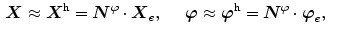
Let  describe the deformation of the body, which transforms referential placements
  to their spatial counterparts
  . Based on this, the deformation gradient is defined as
  which transforms infinitesimal referential line elements
  onto their spatial counterparts
  . Furthermore, let
  and
and  denote an infinitesimal volume element in referential and spatial setting. Accordingly, the Jacobian
  and
and  define the referential and spatial area normals. Then, Nanson’s formula
 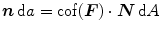 describes the transformation of infinitesimal area elements between the reference and the spatial configuration with the co-factor of
  defined as
 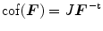 . Fibre-reinforcement of the material is incorporated by assuming two families of fibres to be embedded in the continuum. Their orientation is characterised by referential unit vectors
  ,
,  with
with  .
.
describe the deformation of the body, which transforms referential placements to their spatial counterparts . Based on this, the deformation gradient is defined as which transforms infinitesimal referential line elements onto their spatial counterparts . Furthermore, let and denote an infinitesimal volume element in referential and spatial setting. Accordingly, the Jacobian and define the referential and spatial area normals. Then, Nanson’s formula describes the transformation of infinitesimal area elements between the reference and the spatial configuration with the co-factor of defined as . Fibre-reinforcement of the material is incorporated by assuming two families of fibres to be embedded in the continuum. Their orientation is characterised by referential unit vectors , with .2.2 General Gradient-Enhanced Format of the Free Energy
We assume the local free energy
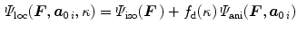
to account for anisotropic non-linear elastic material response under the influence of scalar damage. Basically, we additively compose the effective free energy of the undamaged material of an isotropic contribution  representing the ground substance and of an anisotropic contribution
  associated with
  fibre families. We assume only the anisotropic part to be affected by the damage, whereas the isotropic matrix material remains elastic. In Eq. (1),
  is a scalar internal damage variable, characterising a material stiffness loss of the fibres, while
 ![$$f_\mathrm {d}(\kappa )=1-d\in (0,1]$$](/wp-content/uploads/2016/10/A324942_1_En_2_Chapter_IEq24.gif) represents an appropriate damage function that is at least twice differentiable and satisfies
represents an appropriate damage function that is at least twice differentiable and satisfies  and
and  . This ensures purely elastic behaviour of the undamaged material and complete loss of the related material stiffness for
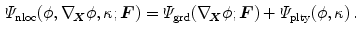
  . Conceptually following the approach by Dimitrijević and Hackl [2], we introduce a gradient-enhanced non-local free energy
  as
as
Here,  contains the referential gradient of the non-local damage field variable
  while
while  incorporates a penalisation term which links the non-local damage variable
  to the local damage variable
  . Consequently, we obtain an enhanced free energy as

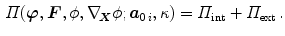
Provided that the external load can be derived from a potential, we can specify the local external energy function as  . In summary, the total potential energy function is additively composed of the internal and external contribution so that its local form reads

(1)
representing the ground substance and of an anisotropic contribution associated with fibre families. We assume only the anisotropic part to be affected by the damage, whereas the isotropic matrix material remains elastic. In Eq. (1), is a scalar internal damage variable, characterising a material stiffness loss of the fibres, while represents an appropriate damage function that is at least twice differentiable and satisfies and . This ensures purely elastic behaviour of the undamaged material and complete loss of the related material stiffness for . Conceptually following the approach by Dimitrijević and Hackl [2], we introduce a gradient-enhanced non-local free energy as(2)
contains the referential gradient of the non-local damage field variable while incorporates a penalisation term which links the non-local damage variable to the local damage variable . Consequently, we obtain an enhanced free energy as(3)
. In summary, the total potential energy function is additively composed of the internal and external contribution so that its local form reads(4)
2.3 Total Potential Energy
The total potential energy of a system additively combines the internal contribution  , reflecting the action of internal forces, and an external contribution
  due to volume and surface forces, i.e.
The internal energy contribution can be written as
while the external contributions, assuming ‘dead’ loads, are provided by
where  denotes the body force vector per unit reference volume and
  characterises the traction vector per unit reference surface area. In this regard, see, for instance, Waffenschmidt and Menzel [15] where a double-layered thick-walled cylindrical tube subjected to internal pressure is analysed on the basis of a total potential.
, reflecting the action of internal forces, and an external contribution due to volume and surface forces, i.e.(5)
(6)
(7)
(8)
denotes the body force vector per unit reference volume and characterises the traction vector per unit reference surface area. In this regard, see, for instance, Waffenschmidt and Menzel [15] where a double-layered thick-walled cylindrical tube subjected to internal pressure is analysed on the basis of a total potential.2.4 Variational Form
The boundary value problem is governed by the principle of minimum potential energy
which requires the first variation of the total potential energy with respect to  and
and  to vanish, i.e.
Taking into account that  and
and  , we obtain a coupled system of variational equations, i.e.
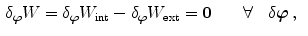
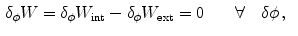
where the internal and external contributions are given in spatial form as
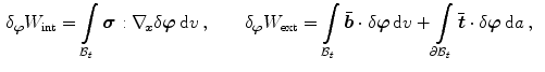
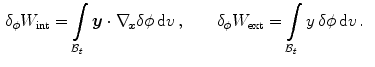
Here the Cauchy stress  and the vectorial damage quantity
  are related to flux terms, whereas the body force
  and the scalar damage quantity
  are associated to source terms. They are defined as
Relations (14) and (15) provide the basis for the finite element discretisation in Sect. 4.
(9)
and to vanish, i.e.(10)
(11)
and , we obtain a coupled system of variational equations, i.e.(12)
(13)
(14)
(15)
and the vectorial damage quantity are related to flux terms, whereas the body force and the scalar damage quantity are associated to source terms. They are defined as(16)
(17)
3 Constitutive Relations
In this section, we first review the hyperelastic constitutive equations adopted on the basis of an isotropic neo-Hookean relation and an anisotropic exponential part. These relations characterise the elastic anisotropic response of the fibre-reinforced material. Secondly, we specify the gradient-enhanced, non-local contribution to the free energy, followed by the continuum damage formulation.
3.1 Hyperelastic Part of the Free Energy
From Sect. 2.2, we recall the local free energy density  , Eq. (1), to be additively composed of an isotropic part
  , representing the isotropic matrix material, and of an anisotropic part
  , representing the individual families of fibres. In the following, we assume the isotropic part to be specified by a compressible neo-Hookean format
![$$\begin{aligned} \varPsi _\mathrm {iso}=\frac{\mu _\mathrm {e}}{2}\left[ I_1-3\right] -\mu _\mathrm {e}\ln (J)+\frac{\lambda _\mathrm {e}}{2}\,[\ln (J)]^2\, , \end{aligned}$$](/wp-content/uploads/2016/10/A324942_1_En_2_Chapter_Equ18.gif)
with  denoting the first invariant. The elastic constants are represented by the Lamé-parameters
  and
and  in terms of the shear modulus
  and the bulk modulus
  . The anisotropic contribution of the local free energy (1) is based on an orthotropic exponential model with two families of fibres including fibre dispersion according to Gasser et al. [5] or Menzel et al. [12], i.e.
![$$\begin{aligned} \varPsi _\mathrm {ani}=\frac{k_1}{2\,k_2}\sum _{i=1}^N\left[ \,\exp \left( k_2\left\langle E_i\right\rangle ^2\right) -1\,\right] \, , \end{aligned}$$](/wp-content/uploads/2016/10/A324942_1_En_2_Chapter_Equ19.gif)
with the strain-like quantity ![$$E_i=\varkappa \, I_1+[1-3\varkappa ]\,I_{4\,i}-1$$](/wp-content/uploads/2016/10/A324942_1_En_2_Chapter_IEq55.gif) and the invariant
and the invariant  for
for  fibre families. The term
  , where
 ![$$\left\langle \bullet \right\rangle =\left[ \left| \bullet \right| +\bullet \right] /2$$](/wp-content/uploads/2016/10/A324942_1_En_2_Chapter_IEq59.gif) is the Macaulay bracket, reflects the assumption that fibres can support tension only. Consequently,
is the Macaulay bracket, reflects the assumption that fibres can support tension only. Consequently, ![$$\varPsi _\mathrm {ani}>0$$” src=”/wp-content/uploads/2016/10/A324942_1_En_2_Chapter_IEq60.gif”></SPAN> only if the fibre-related strain is positive, i.e. <SPAN id=IEq61 class=InlineEquation><IMG alt=]() 0$$” src=”/wp-content/uploads/2016/10/A324942_1_En_2_Chapter_IEq61.gif”>. Fibre dispersion is introduced by means of the parameter
0$$” src=”/wp-content/uploads/2016/10/A324942_1_En_2_Chapter_IEq61.gif”>. Fibre dispersion is introduced by means of the parameter ![$$\varkappa \in [0,\,1/3]$$](/wp-content/uploads/2016/10/A324942_1_En_2_Chapter_IEq62.gif) , where
, where  corresponds to no dispersion, i.e. transverse isotropy, and where
  renders an isotropic distribution. Table 1 summarises the structural and elastic material quantities included in constitutive Eqs. (18) and (19) together with their units. It is important to note that the fibre orientations may be defined arbitrarily, but the present formulation uses only one non-local damage variable so that both fibre families undergo identical degradation. This is physically meaningful as long as both families of fibers possess one and the same stretch history, otherwise a second non-local damage variable should be included in the formulation.
, Eq. (1), to be additively composed of an isotropic part , representing the isotropic matrix material, and of an anisotropic part , representing the individual families of fibres. In the following, we assume the isotropic part to be specified by a compressible neo-Hookean format(18)
denoting the first invariant. The elastic constants are represented by the Lamé-parameters and in terms of the shear modulus and the bulk modulus . The anisotropic contribution of the local free energy (1) is based on an orthotropic exponential model with two families of fibres including fibre dispersion according to Gasser et al. [5] or Menzel et al. [12], i.e.(19)
and the invariant for fibre families. The term , where is the Macaulay bracket, reflects the assumption that fibres can support tension only. Consequently, , where corresponds to no dispersion, i.e. transverse isotropy, and where renders an isotropic distribution. Table 1 summarises the structural and elastic material quantities included in constitutive Eqs. (18) and (19) together with their units. It is important to note that the fibre orientations may be defined arbitrarily, but the present formulation uses only one non-local damage variable so that both fibre families undergo identical degradation. This is physically meaningful as long as both families of fibers possess one and the same stretch history, otherwise a second non-local damage variable should be included in the formulation.Type | Symbol | Description | Unit |
|---|---|---|---|
Structural |  | Fibre orientation vectors | – |
 | Dispersion parameter | – | |
Elastic |  | Shear modulus |  |
 | Bulk modulus |  | |
 | Elastic constant |  | |
 | Elastic constant | – | |
Regularisation |  | Degree of regularisation |  |
 | Penalty parameter |  | |
Damage |  | Saturation parameter |  |
 | Damage threshold |  |
3.2 Gradient-Enhanced Part of the Free Energy
According to Eq. (2), we assume the non-local part of the free energy to be additively composed of a gradient-related term  and of a penalty term
  and specify these terms as
![$$\begin{aligned} \varPsi _\mathrm {grd}(\nabla _{\!\varvec{X}}\phi ; {\varvec{F}}) =\frac{c_\mathrm {d}}{2}\,||\nabla _{\!\varvec{x}}\phi \,||^2 \quad \text {and} \quad \varPsi _\mathrm {plty}(\phi ,\kappa )=\frac{\beta _\mathrm {d}}{2}\,[\phi -\kappa ]^2\, . \end{aligned}$$](/wp-content/uploads/2016/10/A324942_1_En_2_Chapter_Equ20.gif)
The energy-related penalty parameter  approximately enforces the local damage field
  and the non-local field
  to coincide. Furthermore, the gradient parameter
  controls the quasi-non-local character of the formulation and characterises the degree of gradient regularisation:
  results in a local model, while
 ![$$c_\mathrm {d}> 0$$” src=”/wp-content/uploads/2016/10/A324942_1_En_2_Chapter_IEq89.gif”></SPAN> leads to the regularised gradient-enhanced model. The damage-related parameters included in constitutive Eq. (<SPAN class=InternalRef><A href=]() 20) together with their units are summarised in Table 1.
20) together with their units are summarised in Table 1.
and of a penalty term and specify these terms as(20)
approximately enforces the local damage field and the non-local field to coincide. Furthermore, the gradient parameter controls the quasi-non-local character of the formulation and characterises the degree of gradient regularisation: results in a local model, while 3.3 Gradient-Enhanced Damage Model
In order to obtain the stress-like thermodynamic forces driving the local dissipative damage process, we follow the standard Coleman-Noll procedure. Differentiation of the general format of the free energy (3) with respect to time and application of the Clausius-Planck inequality yields, amongst others, a contribution including the thermodynamic force  conjugate to the damage variable
  , i.e.
![$$\begin{aligned} q_\mathrm {loc}=\varPsi _\mathrm {ani}\quad \text {and} \quad q_\mathrm {nloc}=\beta _\mathrm {d}\,[\phi -\kappa ]\,\partial _d\kappa \, . \end{aligned}$$](/wp-content/uploads/2016/10/A324942_1_En_2_Chapter_Equ21.gif)
Furthermore, we adopt the damage condition
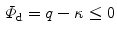
where  refers to the purely elastic loading and
  to damage evolution. Based on the postulate of maximum dissipation, we construct a constrained optimisation problem involving the Lagrange multiplier
  . This results in the following associated evolution equation for the damage variable
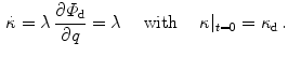
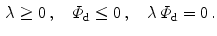
where initiation and termination of damage are governed by the Karush-Kuhn-Tucker complementary conditions
We assume an exponential behaviour for the damage function
![$$\begin{aligned} f_\mathrm {d}(\kappa )=1-d=\exp (\eta _\mathrm {d}\,[\kappa _\mathrm {d}-\kappa ])\, , \end{aligned}$$](/wp-content/uploads/2016/10/A324942_1_En_2_Chapter_Equ25.gif)
with ![$$\eta _\mathrm {d}>0$$” src=”/wp-content/uploads/2016/10/A324942_1_En_2_Chapter_IEq95.gif”></SPAN> so that <SPAN id=IEq96 class=InlineEquation><IMG alt=]() 0$$” src=”/wp-content/uploads/2016/10/A324942_1_En_2_Chapter_IEq96.gif”> and introduce an initial damage threshold
0$$” src=”/wp-content/uploads/2016/10/A324942_1_En_2_Chapter_IEq96.gif”> and introduce an initial damage threshold  , which must be exceeded in order to activate damage evolution. Furthermore, we include a saturation parameter
  . It becomes apparent that larger values of
  accelerate the damage process, whereas larger values of
  lead to a delay of the damage initiation. Note, that for the limiting case
  , damage is initiated from the very beginning of the loading process, whereas damage does not evolve for
  .
.
conjugate to the damage variable , i.e.(21)
(22)
refers to the purely elastic loading and to damage evolution. Based on the postulate of maximum dissipation, we construct a constrained optimisation problem involving the Lagrange multiplier . This results in the following associated evolution equation for the damage variable(23)
(24)
(25)
, which must be exceeded in order to activate damage evolution. Furthermore, we include a saturation parameter . It becomes apparent that larger values of accelerate the damage process, whereas larger values of lead to a delay of the damage initiation. Note, that for the limiting case , damage is initiated from the very beginning of the loading process, whereas damage does not evolve for .4 Finite Element Discretisation
This section deals with the spatial finite element discretisation of the underlying coupled system of non-linear equations. This includes a combination of tri-quadratic serendipity interpolation functions with respect to the displacement field, and tri-linear interpolation functions with respect to the non-local damage field variable where we outline an efficient and compact FE-implementation using a common Voigt-notation-based vector-matrix-format.
4.1 Discretisation
We discretise the domain  by
by  finite elements, so that
  , where every finite element
  is characterised by
  placement-nodes and
  non-local-damage-nodes. According to the isoparametric concept, we interpolate the field variables
  as well as the geometry
  by the same shape functions
by finite elements, so that , where every finite element is characterised by placement-nodes and non-local-damage-nodes. According to the isoparametric concept, we interpolate the field variables as well as the geometry by the same shape functions