, Eugene G. Novikov1, 2, Victor V. Skakun1 and Vladimir V. Apanasovich1
(1)
Department of Systems Analysis and Computer Simulation, Belarusian State University, Minsk, Belarus
(2)
Carl Zeiss Microscopy GmbH, Jena, Germany
Abstract
In this chapter, we describe the global analysis approach for processing time-resolved fluorescence spectroscopy data of molecules in the condensed phase. Combining simultaneous analysis of data measured under different experimental conditions (spatial coordinates, temperature, concentration, emission wavelength, excitation intensity, etc.) with the fitting strategy, enabling parameter linkage and thus decreasing the total amount of estimated variables, makes global analysis more robust and more consistent compared to a sequential fit of single experimental data. We consider the main stages of the global analysis approach and provide some details that are important for its practical implementation. The application of the global approach to the analysis of time-resolved fluorescence anisotropy is demonstrated on experimental data of (enhanced) green fluorescent protein in aqueous solution.
Key words
Global analysisTCSPCTime domainFrequency domainDeconvolution1 Introduction
Structural and dynamical properties of complex, fluorescent biological and chemical systems can be successfully studied using time- and frequency-domain methods of time-resolved fluorescence spectroscopy [1]. The most commonly used time-domain experimental method is time-correlated single-photon counting (TCSPC). In this method the fluorescent sample is excited by a series of short laser pulses of fixed repetition rate and the fluorescence decay is measured and stored in computer memory [1]. Quantitative information about the explored molecular system is obtained by fitting the model-generated decay curve to the experimental sample fluorescence decay. This gives the values of model parameters that characterize the sample under study. In the time-resolved frequency-domain approach [1] the sample is excited by intensity-modulated light at different modulation frequencies. The emission signal of the molecular system is then demodulated and phase-shifted with respect to the modulated excitation light. The dependencies of degree of modulation and phase shift on the modulation frequency are measured and analyzed by the appropriate model to estimate the values of fit parameters characterizing the sample under study.
The experimental methods of time-resolved fluorescence spectroscopy are frequently applied to measure fluorescent molecules in the condensed phase under different experimental conditions such as different temperatures, emission wavelengths, and concentrations. Since some parameters characterizing the investigated molecular system may be independent on the experimental conditions, these sets of data can be simultaneously analyzed using a global analysis approach [2, 3]. The fit parameters that are the same in different experiments are linked and thus kept equal for the corresponding measured curves participating in the fit. The other parameters that change with experimental conditions are fitted independently. As the overall number of fitted parameters decreases, whereas the amount of experimental data remains the same, the global analysis approach has proved to be more robust and more consistent compared to the separate analysis of single curves.
The abilities of the time-resolved fluorescence spectroscopy are significantly extended with introduction of the fluorescence lifetime imaging microscopy (FLIM) technique [1, 4, 5]. This technique uses a wide-field or a confocal microscope to perform the time- or frequency-domain measurements in various spatial points of the sample, thus resolving the immediate molecular environment and the state of a fluorescent molecule in a microscopic image. Another example is the use of genetically encoded fluorescent proteins such as green fluorescent protein (GFP), which can be attached to the protein of interest and expressed in living cells [6]. When two different proteins are labeled with two different variants of GFP, for instance cyan fluorescent protein (CFP) and yellow fluorescent protein (YFP) in living cells, the distance between these proteins when interacting can be mapped in a living cell by using FLIM combined with Förster resonance energy transfer (FRET) [7]. In the following we use the term donor for a protein that is tagged with CFP and the term acceptor for the other protein that is tagged with YFP. In other biosensors donor and acceptor are both linked to a common protein that changes conformation when a ligand is bound and thus alters the donor–acceptor distance. When FRET occurs (i.e., when donor and acceptor are a few nanometers apart) the reaction between excited donor and acceptor in the ground state will decrease the fluorescence lifetime of the donor in various points of the image. The appearance of double-exponential fluorescence intensity decays is frequently encountered because of the presence of a mixture of FRET-active and FRET-inactive donor molecules [8, 9]. To detect the spatially dependent relative contribution of donors participating in FRET global analysis may be applied. The fluorescence intensity decays measured in different points of the image are analyzed globally using double-exponential models. The corresponding fluorescence lifetimes for all space points are linked whereas the pre-exponential factors for each exponent are fitted independently (for an example see ref. 10).
In this chapter we present the main stages required to perform the global analysis of time-resolved fluorescence spectroscopy data. We focus on some practical details important for its implementation. As illustration we show the application of global analysis for fitting the time-resolved fluorescence anisotropy of enhanced GFP from Aequorea victoria (abbreviated as EGFP) in aqueous, buffered solution.
2 Materials
2.1 EGFP
2.2 Time-Resolved Polarized Fluorescence Measurements
Time-resolved fluorescence measurements (20 °C) were carried out using a mode-locked laser pumped by a continuous-wave laser for excitation and TCSPC as the detection technique, as extensively described previously [8, 11, 13]. The samples were excited with plane-polarized light pulses (0.2 ps FWHM) at an excitation frequency of 3.8 MHz and both parallel- and perpendicular-polarized fluorescence intensities were detected.
Experiments with EGFP were conducted at 470-nm excitation and fluorescence detection via the combination of 515-nm cutoff and 512-nm interference filters.
The reference compound for time-resolved fluorescence decay experiments with 470-nm excitation and 512-nm detection was erythrosine B in aqueous solution having a fluorescence lifetime of 85 ps. In all experiments the binning time was 5 ps and 4,096 time channels were used.
3 Methods
3.1 General Global Analysis Algorithm
The global analysis method is based on the simultaneous processing of more than one separately measured data set of a fluorescent species in the condensed phase (see Fig. 1). Such data sets are usually obtained by measuring samples under different experimental conditions (temperature, emission wavelength, excitation intensity, etc.). The application of global analysis becomes meaningful if at least one of the unknown parameters can be assumed to be the same for different measurements. Therefore these parameters, even though being assigned to different experimental data sets, are united into one parameter in the fitting procedure. The global analysis is more robust and consistent than the separate analysis of individual data sets, because it exploits measured information available from several data sets in a more efficient way by reducing the total number of fit parameters.
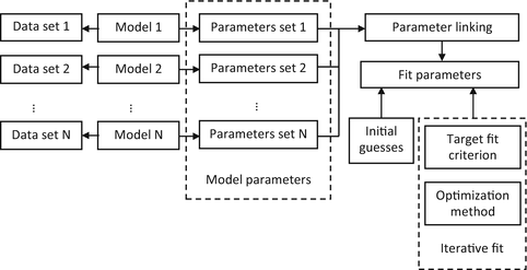

Fig. 1
General scheme of global analysis
The global analysis method can be applied to fit the time-resolved fluorescence data obtained from both time-domain and frequency-domain measurements and includes several consecutive steps.
1.
Collect the data to be analyzed and prepare the data sets. The term “data set” refers to the set of information that can be analyzed by a single mathematical model with a well-defined set of parameters. The data set contains the measured, possibly multidimensional, data from the sample (e.g., fluorescence intensity decay, phase shift, demodulation). In addition, either prior known or experimentally obtained information required for the analysis can also be included.
For time-domain measurements, each data set contains the temporal information (either as time points or as time step and the number of time points), sample fluorescence intensity decay, and either the instrumental response function (IRF, obtained with a scattering solution) or the fluorescence intensity decay of a reference compound with known fluorescence lifetime. The latter is used for deconvolution of measured data (see step 2). A background sample such as solvent alone, obtained at the same conditions as the investigated sample, accounting for impurities or Raman scattering in the sample may also be added to the data set.
For frequency-domain measurements the data set includes the sequence of modulation frequencies and values for phase shift and degree of modulation obtained for each frequency.
Optionally, the data set can include the list of external parameters reflecting the conditions of the measurement (e.g., temperature, excitation/emission wavelength, polarization angle). As these parameters are set by the user during the measurement and are typically known precisely, they can be used by some models as preset (fixed) values to calculate the theoretical curve.
2.
Select the model for each data set created in step 1. Depending on the model, an algorithm should be developed and implemented generating the theoretical curve that is fitted to the measured one.
The analytical models that are applied for fitting the fluorescence intensity decays are based on the following general equations.
If an IRF is used for deconvolution, the basic model for calculating the theoretical decay  takes the form

 takes the form
(1)
where  denotes the instrument response function with a time shift of
  relative to the emission response;
  is the measured intensity of time-dependent background emission contributing with a relative weight of γ; b and c are constant values for dark noise and time-uncorrelated background photons in
  and
and  , respectively; n is the scattered light coefficient and
  represents a model function with the vector of fit parameters
  .
.
 denotes the instrument response function with a time shift of
  relative to the emission response;
  is the measured intensity of time-dependent background emission contributing with a relative weight of γ; b and c are constant values for dark noise and time-uncorrelated background photons in
  and
and  , respectively; n is the scattered light coefficient and
  represents a model function with the vector of fit parameters
  .
.For deconvolution using a single-lifetime reference compound the basic model takes the form


(2)
where  denotes the measured one-exponential reference compound fluorescence intensity decay with decay time
  and δ(t)—Dirac delta-function.
 denotes the measured one-exponential reference compound fluorescence intensity decay with decay time
  and δ(t)—Dirac delta-function.
To complete the model, the function  should be defined. It reflects typical physical processes taking place in the sample under study. A number of models for
  have been published [1, 14, 15]. These include simple models, such as a sum of exponentials or stretched exponential, as well as more complicated ones used in the compartmental formalism.
 should be defined. It reflects typical physical processes taking place in the sample under study. A number of models for
  have been published [1, 14, 15]. These include simple models, such as a sum of exponentials or stretched exponential, as well as more complicated ones used in the compartmental formalism.
One of the most widely used equations for  is the sum of exponential terms:

 is the sum of exponential terms:
(3)
where  and
and  are, respectively, the amplitudes and decay times of corresponding exponents and M is the number of exponents in the sum. The multi-exponential model can be used to fit the fluorescence intensity decays obtained from the mixture of noninteracting species, donor molecules when resonance energy transfer process takes place, etc. [1].
 and
and  are, respectively, the amplitudes and decay times of corresponding exponents and M is the number of exponents in the sum. The multi-exponential model can be used to fit the fluorescence intensity decays obtained from the mixture of noninteracting species, donor molecules when resonance energy transfer process takes place, etc. [1].
The analytical models for fitting the data obtained from frequency-domain measurements are based on the sine  and cosine
  Fourier transforms of the function
  :
:

 and cosine
  Fourier transforms of the function
  :
:
where  is the angular modulation frequency of the excitation light. The general model equations for phase shift
  and degree of modulation
  are
are

 is the angular modulation frequency of the excitation light. The general model equations for phase shift
  and degree of modulation
  are
are
(4)
3.
Link parameters: Every model selected in step 2 contains the set of fit parameters. The term “fit parameter” refers to the value of interest that should be estimated during the analysis. For each fit parameter the range of admissible values can be set by defining the minimum and maximum constraints. The number of fit parameters and their physical interpretation depend on the selected model. The models based on Eqs. 1 and 2 have experiment-specific fit parameters ( for Eq. 1 and
  for Eq. 2) and sample-specific parameters defined by
  . For the multi-exponential model defined by Eq. 3 for time-domain measurements and by Eqs. 5 and 6 for frequency-domain measurements the model-specific parameters are
  and
and  . The fit parameters from all models make up the common list of fit parameters. If for certain parameters the value is known or has been already determined from other, independent experiments, its value can be fixed so that it will remain unchanged during the fit.
 for Eq. 1 and
  for Eq. 2) and sample-specific parameters defined by
  . For the multi-exponential model defined by Eq. 3 for time-domain measurements and by Eqs. 5 and 6 for frequency-domain measurements the model-specific parameters are
  and
and  . The fit parameters from all models make up the common list of fit parameters. If for certain parameters the value is known or has been already determined from other, independent experiments, its value can be fixed so that it will remain unchanged during the fit.
The key feature of the global analysis is the parameter linkage. The linking procedure can be introduced as creating a group of fit parameters that must be kept equal during the fit. The settings (value, minimum, maximum, etc.) of fit parameters included in such group always match the appropriate settings of the group itself. In most cases one parameter group contains the fit parameters that are supposed to have the same value. The linked fit parameters are excluded from the common fit parameter list, whereas the created fit parameter group is added to this common list as a new fit parameter. Since the link procedure replaces several fit parameters in the common list by a group, the total number of parameters to be estimated is reduced. For the analysis to be global, at least one fit parameter group should be created. Generally the number of such global groups is more than one.
4.
 , where
  is the number of data sets. The coefficients
  are functions of the decay times only. As the decay times are linked,
  do not depend on the data set index
  . Coefficients
  depend on both decay times and amplitudes. These coefficients are different for each data set because exponential amplitudes are not linked. Taking into account Eq. 7 the algorithm of the phase plane method can be described as follows.

Initial guess generation: Initial guesses (IG) are required to make the forthcoming iterative fitting procedure fast and reliable. Therefore the IG should be reasonably close to the optimal values of fit parameters that correspond to the best fit of experimental data. If IG are chosen randomly and are located relatively far from the optimal values of fit parameters, the iterative algorithm may converge rather slowly and in some cases may stop untimely, thus leading to biased parameter estimates. To automatically generate the initial guesses a fast non-iterative algorithm should be applied. Such algorithms always take into account the particularity of the models selected for the fit and therefore are not available for any combination of models within global analysis. If such algorithms exist, it is always recommended to use them in combination with the iterative fit routine.
In many practical applications such as FLIM the multi-exponential model can be applied for the global analysis of fluorescence intensity decays [2, 3]. The model is defined by Eqs. 1 and 3, for which the corresponding decay times are assumed to be equal for different data sets and therefore they should be linked, whereas the amplitudes are allowed to be different. If instrumental distortions in Eq. 1 are negligibly small (parameters  equal to 0), the phase plane method can be used to generate initial guesses [16, 17]. It is based on the equivalence of the model given by Eq. 1 with
  defined by Eq. 3 to the following integral equation:

 equal to 0), the phase plane method can be used to generate initial guesses [16, 17]. It is based on the equivalence of the model given by Eq. 1 with
  defined by Eq. 3 to the following integral equation:
(7)
where
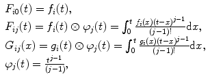

 , where
  is the number of data sets. The coefficients
  are functions of the decay times only. As the decay times are linked,
  do not depend on the data set index
  . Coefficients
  depend on both decay times and amplitudes. These coefficients are different for each data set because exponential amplitudes are not linked. Taking into account Eq. 7 the algorithm of the phase plane method can be described as follows.
(a)
Calculate integral functions  and
and  . Since in practice
  and
and  are obtained on discrete set of time points
  the integration is replaced by summation and discrete convolution of
  and
and  with
with  is calculated giving
  and
and  .
.
 and
and  . Since in practice
  and
and  are obtained on discrete set of time points
  the integration is replaced by summation and discrete convolution of
  and
and  with
with  is calculated giving
  and
and  .
.(b)
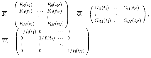
For each data set construct the following matrices:

(c)
Obtain the vector of coefficients  by the linear least-squares method. To do this prepare for each data set the matrices:

 by the linear least-squares method. To do this prepare for each data set the matrices:
(8)
Find the coefficients  by solving the system of linear equations. This solution in matrix form can be represented as follows:

 by solving the system of linear equations. This solution in matrix form can be represented as follows:
(9)
where  is a vector of coefficients
  ; matrices
  and
and  are obtained from matrix
  :
:

 is a vector of coefficients
  ; matrices
  and
and  are obtained from matrix
  :
:
(d)
Get Clinical Tree app for offline access
Calculate estimations for decay times as roots of the following polynomial:


