, Anatoli V. Digris1 and Vladimir V. Apanasovich1
(1)
Department of Systems Analysis and Computer Simulation, Belarusian State University, Minsk, Belarus
Abstract
In fluorescence correlation spectroscopy (FCS) and photon counting histogram (PCH) analysis, the same experimental fluorescence intensity fluctuations are used, but each analytical method focuses on a different property of the signal. The time-dependent decay of the correlation of fluorescence fluctuations is measured in FCS yielding molecular diffusion coefficients and triplet-state parameters such as fraction and decay time. The amplitude distribution of these fluctuations is calculated by PCH analysis yielding the molecular brightness. Both FCS and PCH give information about the molecular concentration. Here we describe a global analysis protocol that simultaneously recovers relevant and common parameters in model functions of FCS and PCH from a single fluorescence fluctuation trace. Application of a global analysis approach allows increasing the information content available from a single measurement that results in more accurate values of molecular diffusion coefficients and triplet-state parameters and also in robust, time-independent estimates of molecular brightness and number of molecules.
Key words
Fluorescence fluctuation spectroscopyFluorescence correlation spectroscopyPhoton counting histogramFluorescence intensity distribution analysisGlobal analysis1 Introduction
Fluorescence correlation spectroscopy (FCS), originally introduced by Elson et al. [1–3] in the early 1970s, has become a widely used technique for studying various dynamic molecular processes. It has found applications in measuring local concentrations, mobility coefficients, reaction rates, and detection of intermolecular interactions in vitro and in vivo [4–7]. The sensitivity and noninvasive nature of FCS has made it an important technique for studying molecular processes in cells and thus a useful tool for biochemists, biophysicists, and biologists. After developing new data analysis methods, this technique was renamed to a more general term: fluorescence fluctuation spectroscopy (FFS).
Fluorescence fluctuation methods are based on the detection of tiny, spontaneous fluctuations in fluorescence intensity caused by deviations from thermal equilibrium in an open system. These fluctuations can arise, e.g., because of diffusion of fluorescent molecules in and out of a well-defined observation volume generated by a focused laser beam. The intensity fluctuations can be monitored and autocorrelated over time as in fluorescence correlation spectroscopy [6, 8] or a distribution of photon counts can be analyzed as in photon counting histogram (PCH) analysis [9, 10] or in fluorescence intensity distribution analysis (FIDA) [11, 12].
Performing fluorescence fluctuation spectroscopy experiments is relatively straightforward. However, the theory for FFS is based on several assumptions, which do not always hold in a real experimental situation. For example, FFS analysis assumes that the experimental observation volume has a Gaussian shape, which is not always true especially for in vivo measurements [13]. Dead time and afterpulsing of the photodetectors may influence FIDA and PCH analysis [14]. There are a number of optical factors that influence FFS measurements such as cover-slide thickness, refractive index of the sample and optical saturation that should be taken into account for proper analysis [15, 16]. In a confocal microscope configuration employing one-photon excitation, a PCH model with a three-dimensional Gaussian observation volume profile does not adequately fit the experimental fluorescence fluctuation data [17, 18]. In addition, there is a clear effect of bin time on FIDA and PCH analysis, which influences the estimation of molecular concentration and brightness [19, 20]. While it is crucial that the experimental setup must be optimized to be close to ideal conditions, one should also be aware of all these factors in the data analysis procedure to avoid erroneous fits and misinterpretation of the experimental data.
Dependence of model parameters in PCH and FIDA on the bin time makes it difficult to recover the true time-independent brightness and number of molecules from just a single measured photon counting distribution (PCD). PCD refers here to the measured and theoretical distribution of photon counts, while PCH is a commonly used term to denote the method of analysis. An attempt to fit PCD calculated at a very small bin time to avoid any influence of diffusion and triplet kinetics usually fails if the detected photon count rate is not high enough. The PCD calculated at such conditions has only a few data points, which makes it difficult to fit the data well. To get time-independent brightness and number of molecules from a fit of PCD calculated at higher bin time, knowledge of diffusion and triplet parameters is required [19, 20].
A number of extensions of PCH and FIDA methods enabling simultaneous determination of diffusion coefficients and brightness of molecules were proposed up to this time: fluorescence intensity multiple distribution analysis (FIMDA) [19], photon counting multiple histogram (PCMH) analysis [20], master equations fluorescence intensity distribution analysis (ME-FIDA) [21], and the method, originated from the numerical solution of the diffusion equation [22].
The fit of a set of PCDs calculated at different bin times in FIMDA [19] or PCMH analysis [20] enables recovering of all parameters (including diffusion times, triplet fraction and decay time) from a single analysis. However, both FIMDA and PCMH have a drawback. These methods use the correction in the form of an integral of the time-dependent part of the FCS model. It means that the same correction value can be achieved for a different functional form of the integrand; for example, one can set the diffusion time to a very small value and compensate this by appropriate value of triplet parameters and vice versa. Therefore, after global analysis of several PCDs, the fit can be satisfactory, but results in erroneous values for diffusion, triplet, and (also) other parameters.
Although it is well possible to analyze FFS data separately by original FCS and PCH/FIDA methods or their extensions and to estimate all parameters of interest, it is advantageous to combine the complementary FFS methods in a global analysis and to increase the information content available from a single measurement. FCS has been established as a robust method for estimation of triplet parameters (fraction and decay time) and diffusion times (or coefficients) [8]. Vice versa, after correcting for the bin-time effect (using obtained estimates of triplet and diffusion parameters), PCH/FIDA analysis yields correct time-independent estimates for the brightness that finally helps to obtain correct concentrations in FCS, if the sample contains two (or more) components having different brightness values. Global analysis of ACF and PCD increases sensitivity and accuracy of the analysis while keeping the total number of fit parameters almost unchanged. Therefore, it results in more accurate values of triplet-state and diffusion parameters and also in robust, time-independent estimates of molecular brightness and number of molecules for a relatively broad range of measurement conditions.
The growing number of applications of FFS methods demands for new approaches in data processing, aiming at increased speed and robustness. Iterative algorithms of parameter estimation, although proven to be universal and accurate, require some initial guesses (IG) for the unknown parameters. If the IG are in close proximity to the optimal values of unknown parameters, they can significantly increase the efficiency and accuracy of the fit. If the target criterion surface has a complex shape with many local minima, the possibility to reach the global minimum directly depends on the quality of IG. Being an essential component of any data processing technology, IG become especially important in case of PCH/FIDA, since even with apparently reasonable, and physically admissible but randomly chosen IG, the iterative procedure may converge to situations where for a certain combination of parameters, the PCH/FIDA model cannot be numerically evaluated [23]. Iterative fitting with generated IG proved to be more robust and at least five times faster than with an arbitrarily chosen IG [23]. It is also important that a reliable algorithm of IG generation reduces user participation and thereby leads to a more standardized and automated procedure.
In this chapter we describe the global analysis protocol of ACF and PCD. The use of the method is demonstrated through fitting of experimental fluorescence fluctuation data obtained from monomeric and dimeric forms of enhanced green-fluorescent protein (eGFP) in aqueous buffer.
2 Materials
2.1 Samples
Monomeric and dimeric eGFP were purified according to a recently described procedure [24]. The two eGFP molecules in the dimer were linked by six amino acids (GSGSGS). Purified monomeric and dimeric eGFP solutions were in 50 mM TRIS buffer (pH 8.0). For the measurements, 200-μl solutions were added to an 8-chambered cover glass (Lab-Tek, Nalge Nunc International Corp., USA). Rhodamine 110 (R110) (Invitrogen) in water was used for calibration measurements.
2.2 Instrumentation
The measurements were performed on the ConfoCor 2-LSM 510 combination setup (Carl Zeiss, Jena, Germany) detailed in [25–27]. eGFP was excited with the 488 nm line from an argon-ion laser (excitation intensity in the range 10–40 μW) focused into the sample with a water immersion C-Apochromat 40× objective lens N.A. 1.2 (Zeiss). After passing through the main beam splitters HFT 488/633, the fluorescence was filtered with a band pass 505–550 and detected with an avalanche photodiode (APD). The pinhole for confocal detection was set at 70 μm. The microscope was controlled by Zeiss AIM 3.2 software. Raw intensity fluctuation data consisting of up to 4 × 10⁶ photons were collected from single measurements. The data collection time ranged between 30 and 120 s.
3 Methods
Global analysis of ACF and PCD is performed by the iterative least-squares method with the Marquardt-Levenberg optimization [28] (see details of its realization in Chapter 10 by Digris et al. in the same volume). To successfully apply it in the analysis of ACF and PCD, one has to know:
1.
How to calculate the FCS model?
2.
How to calculate the PCH model?
3.
How to generate initial guesses for fit parameters?
4.
How to perform the linking of fit parameters?
5.
Which criterion to use to stop the fit?
Answers to these questions are given in the subsequent subsections.
3.1 Calculation of the FCS Model
The FCS model is calculated using the general form
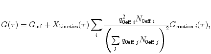
where  , N 0eff is the number of molecules in the effective volume
  ,
, ![$$ {\chi_k}=\int\nolimits_V {{{{[{{{B(\mathbf{ r})}} \left/ {{{B_0}}} \right.}]}}^k}\mathrm{ d}V} $$](/wp-content/uploads/2017/03/A299540_1_En_33_Chapter_IEq00333.gif) , q 0eff is the specific brightness of molecules (in photon counts per second per molecule),
, q 0eff is the specific brightness of molecules (in photon counts per second per molecule),  denotes a kinetic process, and
  describes the type of motion of the particles. Subscript 0 denotes that the given parameter does not depend on time. B(r) is the brightness profile function, which is the product of excitation intensity and detection efficiency. The kinetic process and type of motion depend on the experimental conditions.
(1)
, N 0eff is the number of molecules in the effective volume , , q 0eff is the specific brightness of molecules (in photon counts per second per molecule), denotes a kinetic process, and describes the type of motion of the particles. Subscript 0 denotes that the given parameter does not depend on time. B(r) is the brightness profile function, which is the product of excitation intensity and detection efficiency. The kinetic process and type of motion depend on the experimental conditions.To demonstrate the application of the global analysis method, we used the model describing L independent molecular species diffusing freely in a 3D-Gaussian-shaped observation volume and undergoing singlet-triplet transitions [29]:
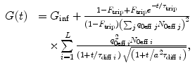
where F trip and τ trip are, respectively, the fraction and the relaxation time of molecules in the triplet state,  , ω 0 and z 0 are, respectively, the lateral and axial radii of the confocal detection volume, and τ diff is the lateral diffusion time, which is related to the diffusion coefficient D tran via τ diff = ω 0 2/(4D tran). All molecules are supposed to have the same triplet-state parameters.
(2)
, ω 0 and z 0 are, respectively, the lateral and axial radii of the confocal detection volume, and τ diff is the lateral diffusion time, which is related to the diffusion coefficient D tran via τ diff = ω 0 2/(4D tran). All molecules are supposed to have the same triplet-state parameters.3.2 Calculation of the PCH Model
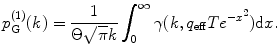
In contrast to the FCS model, which is represented by a relatively simple equation, the PCH model does not have a closed-form solution. It is calculated by a numerical algorithm that includes several steps. Here we describe the algorithm that calculates the PCD P(k) via successive convolutions of single-molecular PCD  [9]. This algorithm allows accurately calculating the PCD using a wide range of model parameters, whereas other algorithms [11, 30] fail to calculate the model due to various numerical problems. The algorithm steps are described below (see Note 1 for details):
[9]. This algorithm allows accurately calculating the PCD using a wide range of model parameters, whereas other algorithms [11, 30] fail to calculate the model due to various numerical problems. The algorithm steps are described below (see Note 1 for details):1.
Calculate the PCD 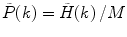 , where
  is the measured photon counting histogram and M is the total number of bins that can be readily calculated from the histogram itself:
  , if
, if  decays to zero.
, where is the measured photon counting histogram and M is the total number of bins that can be readily calculated from the histogram itself: , if decays to zero.2.
Calculate the binning correction factor B 2(T) for each diffusion component as
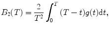
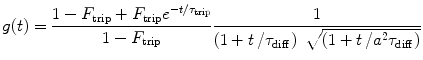
where T is the counting time interval (bin time), g(t) is a time-dependent term of the autocorrelation function in FCS
(3)
(4)
and a, F trip, τ trip, τ diff are fit parameters. The integral in Eq. 3 is calculated numerically as a sum of two integrals (from 0 to t br and from t br to T) by the function qadrat [31]. The value of t br is calculated as a minimum of function:  , where
  . The minimum of function can be calculated, e.g., by the function mimin [31].
, where . The minimum of function can be calculated, e.g., by the function mimin [31].3.
Calculate  ,
,  , where q 0eff and N 0eff are fit parameters, for each brightness component (for the sake of simplicity we omitted subscripts, which denote the component index). For a multicomponent system where each brightness component has a different molecular weight, the correction should be calculated using the proper diffusion component.
, , where q 0eff and N 0eff are fit parameters, for each brightness component (for the sake of simplicity we omitted subscripts, which denote the component index). For a multicomponent system where each brightness component has a different molecular weight, the correction should be calculated using the proper diffusion component.4.
Calculate the single-molecular PCD  for each brightness component:
![$$ {p^{(1) }}(k)=\frac{{1+{F_2}}}{{{{{(1+{F_1})}}^2}}}\left[ {p_{\mathrm{ G}}^{(1) }(k)+\frac{1}{{k!\Theta}}\sum\limits_{n=k}^{\infty } {\frac{{{(-1)^{n-k }}{{{({q_{\mathrm{ eff}}}T)}}^n}{F_n}}}{{(n-k)!{(2n)^{{{3 \left/ {2} \right.}}}}}}} } \right], $$](/wp-content/uploads/2017/03/A299540_1_En_33_Chapter_Equ00335.gif)
where F n , n = 1, 2 are instrumental out-of-focus correction parameters (F n are fit parameters) and
for each brightness component:(5)
(6)
The incomplete gamma function  is calculated as described in [32] (gammp) and the infinite integral is calculated as a sum of two definite integrals (from 0 to 2.4 and from 2.4 to 20). The integration limits were defined empirically by investigating the behavior of the integrand for many combinations of its parameters. The additional integral was added to ensure the acceptable accuracy of the integration if the integrand does not decay to zero at 2.4. Integration is performed numerically by the function qadrat [31]. The parameter Θ is varied depending on the product of q eff and T. We define empirically: if(q eff T < 10) Θ = 1; else if(q eff T < 50) Θ = 6; else if(q eff T < 100) Θ = 12; else Θ = 20;
is calculated as described in [32] (gammp) and the infinite integral is calculated as a sum of two definite integrals (from 0 to 2.4 and from 2.4 to 20). The integration limits were defined empirically by investigating the behavior of the integrand for many combinations of its parameters. The additional integral was added to ensure the acceptable accuracy of the integration if the integrand does not decay to zero at 2.4. Integration is performed numerically by the function qadrat [31]. The parameter Θ is varied depending on the product of q eff and T. We define empirically: if(q eff T < 10) Θ = 1; else if(q eff T < 50) Θ = 6; else if(q eff T < 100) Θ = 12; else Θ = 20;5.
Calculate  .
.
.6.
Calculate P(k) for each brightness component:
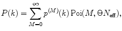
where  is M-times convolution of the single-molecule PCD and Poi(k,η) denotes the Poisson distribution with the mean value η. Do it in a recurrent way: set all elements in the array P(k) to zero; at M = 0 calculate
  and
and  multiply results, and add the product to the sum; at M = 1 calculate
  , multiply the result to
  , and add the product to the sum; at M = 2, 3, … calculate
  , perform a convolution
  , multiply the results, and add the product to the sum. Stop the calculation of the sum when
  after reaching its maximum. Such recurrent calculation of both Poisson distribution and M-times convolution increases the computation efficiency of the algorithm.
(7)
is M-times convolution of the single-molecule PCD and Poi(k,η) denotes the Poisson distribution with the mean value η. Do it in a recurrent way: set all elements in the array P(k) to zero; at M = 0 calculate and multiply results, and add the product to the sum; at M = 1 calculate , multiply the result to , and add the product to the sum; at M = 2, 3, … calculate , perform a convolution , multiply the results, and add the product to the sum. Stop the calculation of the sum when after reaching its maximum. Such recurrent calculation of both Poisson distribution and M-times convolution increases the computation efficiency of the algorithm.7.
Calculate the total PCD. The PCD of a number of independent species is given by a convolution of PCD of each species

(8)
8.
Perform the final convolution of the obtained P(k) with the background term
where λ is the background count rate (fit parameter), if necessary.
(9)
9.
Perform the correction on afterpulses and dead time if necessary. Correction on afterpulses and dead time can be made according to the algorithm described in [21]. Correction for afterpulses is done by the following formula:
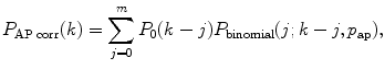
where p ap is the afterpulsing probability, m is a number of points in PCD, P 0(k) is the ideal PCD (i.e., without the correction), and P binomial is the binomial distribution
(10)
(11)
This algorithm works well, if afterpulses are always counted in the same bin together with the main events. This assumption is satisfied for avalanche photodiodes where afterpulses are delayed on a relatively short time (25–40 ns). Correction for dead time is done by the following formula:
where τ dt is the detector dead time. Parameters p ap, τ dt are fit parameters.
(12)
3.3 Generation of Initial Guesses in Photon Counting Histogram Analysis
Here we describe the efficient algorithm of generation of initial guesses for “main” parameters (q 0eff i and N 0eff i , i = 1,2 and F 1, F 2) of one- and two-component PCH models:

1.
Calculate the first four cumulants  of the measured PCD. The experimental fluorescence factorial cumulants are calculated through fluorescence factorial moments
where  is a measured PCD and the angular brackets indicate averaging with the set of probabilities
  . If a photon counting histogram
  is measured instead of PCD
  , one must perform the normalization:
  .
.
of the measured PCD. The experimental fluorescence factorial cumulants are calculated through fluorescence factorial moments (13)
(14)
is a measured PCD and the angular brackets indicate averaging with the set of probabilities . If a photon counting histogram is measured instead of PCD , one must perform the normalization: .2.
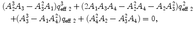
For the case of a one-component model, calculate IG using equations summarized in Table 1 (see Note 2 for details).
Table 1
Initial guesses for PCH analysis for a one-component system
Parameter fixing | IG |
|---|---|
λ, F 1, F 2 are fixed |  , , 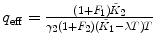 |
F 1, F 2 are fixed | 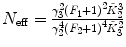 , ,  , , 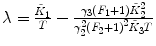 |
λ, F 1 are fixed |  , , 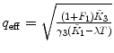 , , 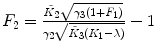 |
λ, F 2 are fixed | 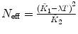 , , 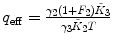 , , 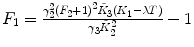 |
λ is fixed |  , ,  , , 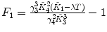 , , 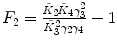 |
4.
Calculate the time-independent estimates of brightness and number of molecules: 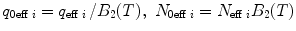 . Do it independently for each brightness component using diffusion parameters from the proper diffusion component.
. Do it independently for each brightness component using diffusion parameters from the proper diffusion component.5.
Get Clinical Tree app for offline access
For a two-component model with known background λ and known instrumental parameters F 1, F 2, the system of nonlinear equations (Eq. 37) (see Note 2 for details) can be reduced to a third-order polynomial with respect to q eff 2