Fig. 10.1
Flow chart for sequential trend testing
The advantage of trend testing methods is that for monotonic dose–response patterns, the methods are more sensitive than pairwise comparisons alone. Note that the NOSTASOT for a particular endpoint is being declared based on a lack of statistical significance, which could result due to lack of a true effect, or due to a lack of power to detect an effect.
There are several options for implementing trend testing. One common approach is to estimate linear contrasts in the context of an ANOVA. Consider the data shown in Table 10.1 and Fig. 10.2 for the liver enzyme alanine aminotransferase (ALT) from a hypothetical 1-month general toxicology study. Elevations in ALT often reflect changes in liver structure or function.
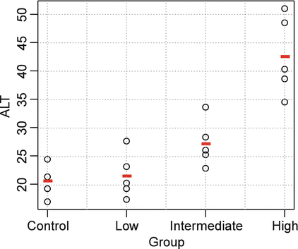

Fig. 10.2
Scatterplot of example ALT data
Table 10.1
Example hypothetical ALT (U/L) data from a 1-month general toxicology study in rats
Control | Low dose | Intermediate dose | High dose |
|---|---|---|---|
21.3 | 17.3 | 33.6 | 40.3 |
16.9 | 20.2 | 22.8 | 48.5 |
24.4 | 23.1 | 28.3 | 34.5 |
19.2 | 27.6 | 25.2 | 38.6 |
21.3 | 19.2 | 26.0 | 51.0 |
The data suggest an elevation in ALT levels with increasing dose. Note also that variation appears to increase with the magnitude of ALT. This is common for many clinical pathology parameters, and a log transformation is often appropriate. For this example, Levene’s Test didn’t suggest strong evidence of unequal variance (p = 0.085), and hence we analyze the data on the original scale. The overall F-test from an ANOVA indicates a significant difference among the groups (F = 23, p < 0.001, df = 3.16). The toxicologist is specifically interested in which dose groups differ from control, and so pairwise comparisons are conducted. Table 10.2 shows the results of pairwise comparisons using Dunnett’s Test and a sequential trend test.
Table 10.2
Summary of pairwise comparisons for ALT
P-value | |||||
|---|---|---|---|---|---|
Treatment | N | Mean | SD | Dunnett | Trend |
Control | 5 | 20.6 | 2.8 | – | – |
Low | 5 | 21.5 | 4.0 | 0.98 | 0.39 |
Intermediate | 5 | 27.2 | 4.1 | 0.10 | 0.02 |
High | 5 | 42.6 | 6.9 | <0.01 | <0.01 |
Table 10.3 shows the linear contrasts used for the trend test. Contrast 1 tests for an overall linear trend among all four dose groups. Contrast 2 tests for a linear trend among the control, low, and intermediate dose groups only, and it is only conducted if Contrast 1 is statistically significant. Similarly, Contrast 3 tests for a difference between the control and low dose group and is only conducted if Contrast 2 is statistically significant. For these data, both the high and intermediate doses would be declared significantly different from control, at the 5 % level. Note that using this sequential approach, testing at subsequent doses only occurs if the initial contrast is statistically significant. Hence, the overall (i.e., family-wise) error rate of the procedure is less than or equal to α.
Table 10.3
Linear contrasts for trend testing with four treatment groups
Contrast 1 | Contrast 2 | Contrast 3 | |
|---|---|---|---|
Control | −3 | −1 | −1 |
Low | −1 | 0 | 1 |
Intermediate | 1 | 1 | 0 |
High | 3 | 0 | 0 |
In contrast, Dunnett’s Test indicates a difference between the high dose group and control only, at the 5 % level. In general, in settings where monotonic dose–response patterns are expected, then trend testing methods will be more powerful than Dunnett’s Test. Simulations can be used to assess the extent of the advantage. For example, assume that the true mean levels of ALT are (21,24,26,29) in the control, low dose, intermediate dose, and high dose groups respectively, and that our estimate (from historical control data) of the standard deviation is 6. For a range of sample sizes, Table 10.4 shows the proportion of times the high dose group was significantly different from the control group at the 5 % level.
Table 10.4
Power to detect differences between high dose group and control using sequential trend test and Dunnett’s test
N per group | Power – Trend test (%) | Power – Dunnett’s test (%) |
|---|---|---|
3 | 32.0 | 17.4 |
4 | 42.7 | 25.9 |
5 | 52.9 | 33.8 |
6 | 61.2 | 42.3 |
7 | 70.0 | 51.6 |
8 | 75.7 | 58.5 |
9 | 80.4 | 63.9 |
10 | 84.4 | 69.2 |
15 | 96.1 | 89.5 |
20 | 98.9 | 96.2 |
In addition to the linear contrasts approach, there are other methods for testing for trends. For example, some methods assume only a monotonic response. The null and alternative hypotheses in this setting are:

 with at least one strict inequality. One method due to Williams (1971, 1972) is basically a series of pairwise t-tests of each dose group versus control, based on amalgamated means. Because of this similarity to the traditional t test, it was termed the
  test. The amalgamation procedure enforces a non-decreasing (or non-increasing) ordering of the sample means, using the pooled adjacent violators (PAV) algorithm Consider an example where the dose group means are (2,4,6,5) as shown in Fig. 10.3. The PAV algorithm moves left to right, checking for non-monotonicity among adjacent pairs. In this case, the intermediate and high dose groups violate monotonicity, so their means are averaged. The final group means are thus (2,4,5.5,5.5). In a second more extreme example, assume that the dose group means are (2,7,7,1), as shown in Fig. 10.4. In this case, the intermediate and high dose group means violate monotonicity, and so their means are pooled, resulting in group mean equal to (2,7,4,4). Because the low dose group mean now violates monotonicity when compared to the pooled intermediate and high dose group means, those three group means are pooled, resulting in (2,5,5,5) for the final amalgamated group means. In addition to the pairwise t-tests based on amalgamated means due to Williams, there is also a trend test based on amalgamation means. This test, called the
  test (Barlow et~al. 1972).is essentially an overall ANOVA F-test based on amalgamated means. For more details on the
  and
and  tests, including critical values and calculation of p-values, see the original papers, as well as Bailey (1998).
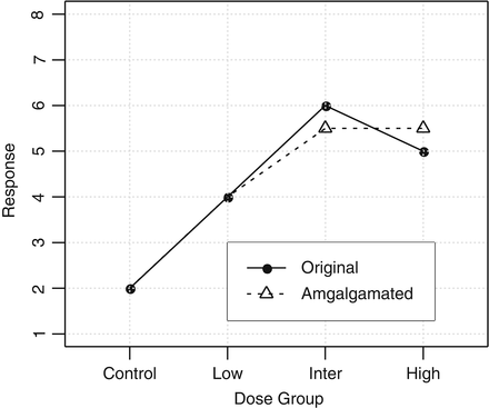
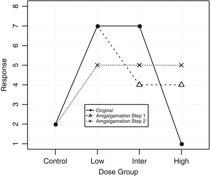


 test. The amalgamation procedure enforces a non-decreasing (or non-increasing) ordering of the sample means, using the pooled adjacent violators (PAV) algorithm Consider an example where the dose group means are (2,4,6,5) as shown in Fig. 10.3. The PAV algorithm moves left to right, checking for non-monotonicity among adjacent pairs. In this case, the intermediate and high dose groups violate monotonicity, so their means are averaged. The final group means are thus (2,4,5.5,5.5). In a second more extreme example, assume that the dose group means are (2,7,7,1), as shown in Fig. 10.4. In this case, the intermediate and high dose group means violate monotonicity, and so their means are pooled, resulting in group mean equal to (2,7,4,4). Because the low dose group mean now violates monotonicity when compared to the pooled intermediate and high dose group means, those three group means are pooled, resulting in (2,5,5,5) for the final amalgamated group means. In addition to the pairwise t-tests based on amalgamated means due to Williams, there is also a trend test based on amalgamation means. This test, called the
  test (Barlow et~al. 1972).is essentially an overall ANOVA F-test based on amalgamated means. For more details on the
  and
and  tests, including critical values and calculation of p-values, see the original papers, as well as Bailey (1998).
Fig. 10.3
Example of amalgamation procedure

Fig. 10.4
Example of multiple-step amalgamation procedure
Occasionally in general toxicology studies, the observed pattern in group means with increasing dose is not monotonic. See, for example, data shown in Fig. 10.5. In these cases, sequential trend testing methods lead to one of two conclusions. In one case, the initial trend test will not be significant, so the sequential testing stops with no dose groups being declared different from control. In a second case, the initial trend test across all dose groups will be significant (due to the influence of the low and intermediate dose groups), leading to the high dose group being declared significant. In the case shown in Fig. 10.3, the initial trend test (using linear contrasts) is significant (p = 0.016), leading to the conclusion that the high dose group differs from control. In either of the two cases, interpretation can be challenging. One way of addressing this issue is to include a check for monotonicity upfront. One approach to testing for non-monotonicity is based on comparing the group means with the amalgamated means, using an F-test. See Healey (1999) for more details. If there is evidence of non-monotonicity, then the results from pairwise comparisons (say, using Dunnett’s Test) could be provided instead. Alternatively, the approach taken by Bretz and Hothorn (2003) could be considered, in which multiple contrast tests (MCT’s) are used to identify a potential trend only up to a given dose level.
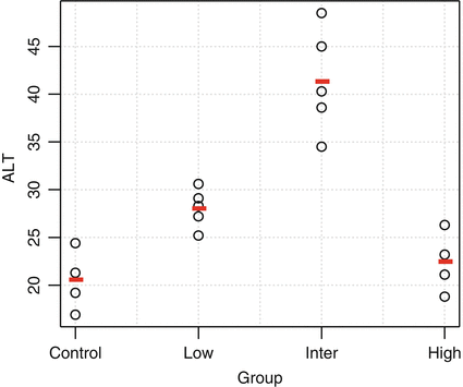

Fig. 10.5
Example of non-monotonic relationship with dose group
10.2.2.2 Parametric vs. Nonparametric Methods
In a typical statistical comparison of groups (e.g., using an ANOVA model), the researcher checks (often visually) distributional assumptions such as normality of the residuals and equal variability across treatment groups. Depending on the assessment, it might make sense to transform the dependent variable (e.g., log) or use a nonparametric approach. However, in the analysis of general toxicology studies, the statistical methods are often implemented as part of automated systems; the same model will be run for multiple endpoints, possibly across multiple timepoints. Hence, it may not be feasible to check data distributions and other assumptions for each model at the time of analyses. There are at least three approaches to handling this issue.
One approach is to automate the assessment of the distributional or other assumptions prior to analysis. This approach is often represented as a “decision tree” (not to be confused with classification and regression trees used in predictive modeling) or flow chart. For example, depending on an initial test of normality, the data may or may not be rank transformed, or undergo some other transformation, prior to analysis. Note that in some systems we have encountered, data are analyzed nonparametrically if an initial test suggests a departure from the assumption of constant variability across treatment groups. Many nonparametric approaches (e.g., Wilcoxon, Kruskal–Wallis) still rely on the homogeneous variance assumption, however. A second approach is to evaluate historical control data to evaluate the distribution of each endpoint. Those variables that deviate appreciably from normality could be routinely analyzed using a log or rank transformation; these choices for each endpoint would be prespecified in the automated system. A third approach is to use a rank transformation for all parameters. This would guard against cases where an extreme value may mask a potential effect, and in general won’t result in an appreciable loss of power. For example, using the setup in the previous section, with mean ALT equal to (21, 24, 26, 29), we can compare the power of a rank-based approach to the original, using the sequential trend test based on linear contrasts. The results are shown in Table 10.5 and suggest some loss of power with the rank-based approach, but typically only a few percentage points in this scenario.
Table 10.5
Power comparison of parametric and rank-based sequential trend tests
Based on original data values | Based on ranks | |||||
|---|---|---|---|---|---|---|
N per group | Low dose (%) | Intermediate dose (%) | High dose (%) | Low dose (%) | Intermediate dose (%) | High dose (%) |
3 | 15.6 | 24.4 | 32.0 | 15.9 | 24.9 | 31.7 |
4 | 17.7 | 30.0 | 42.7 | 17.9 | 30.0 | 41.3 |
5 | 19.3 | 35.4 | 52.9 | 18.7 | 34.4 | 50.4 |
6 | 21.6 | 39.6 | 61.2 | 21.2 | 39.2 | 58.9 |
7 | 23.0 | 45.4 | 70.0 | 22.9 | 44.7 | 67.6 |
8 | 26.4 | 49.6 | 75.7 | 26.0 | 48.7 | 73.0 |
9 | 27.5 | 53.6 | 80.4 | 26.7 | 53.1 | 78.0 |
10 | 29.4 | 57.0 | 84.4 | 28.5 | 56.4 | 82.7 |
15 | 38.2 | 73.0 | 96.1 | 37.4 | 71.6 | 95.2 |
20 | 47.6 | 83.5 | 98.9 | 46.5 | 82.3 | 98.6 |
10.2.2.3 Sex Effects
General toxicology studies are typically conducted in both sexes. Traditionally, statistical analyses have been conducted separately for each sex. There may be a gain in sensitivity by conducting a combined analysis including a model term for sex (i.e., as a block) in the ANOVA. The challenge arises if there is a statistical interaction between sex and dose for one or more parameters in a given study. It is not uncommon to observe sex-related differences in exposure due to differential metabolism or hormonal influence. In this case, the toxicologist will want to evaluate the impact of treatment separately for each gender. Again, since these analyses are often automated, the conventional approach has been to assume the potential for an interaction, and analyze by gender. This is an area for continued development.
10.2.2.4 Time Effects
Some endpoints, such as organ weights, can be collected only once in a general toxicology study. Others, such as body weights and food intake, are captured more frequently (e.g., weekly). Clinical chemistry, hematology, and urinalysis parameters are typically collected at the end of study, but may also be collected multiple times (e.g., monthly in a 3-month study). In some cases, and especially for large animal studies (e.g., NHP, dog), a baseline measurement (i.e., prior to any dosing) may be taken for each animal. In these studies, it is typical for the toxicologist and/or clinical pathologist to focus on changes from baseline values, rather than comparing control and test article-administered animals at each time point, especially when the sample sizes are small (e.g. 3/sex/group).
Incorporating a baseline adjustment (i.e., as a covariate) into an ANOVA model may, in some cases, improve the power of these analyses. However, it is important to evaluate the extent of correlation between baseline and follow-up measurements for each endpoint. A recent internal Pfizer study of clinical pathology control data from 20 GLP general toxicology studies in NHP’s showed a substantial range in correlation (approximately 0.15–0.95) across about 45 endpoints. Some endpoints (e.g., ALT) had within-animal correlations above 0.90. Others (e.g., glucose) were in the range of 0.35. Overall, more than 1/3 of the endpoints had within-animal correlations below 0.5; for these endpoints, including a baseline covariate may actually reduce the sensitivity of statistical tests.
10.2.2.5 Reference Ranges
In addition to comparisons between dose groups and concurrent controls in a general toxicology study, for many endpoints there are well-established reference ranges, based on historical control data, against which to compare individual data values. A reference range is defined as an interval in which some percentage (e.g. 95 %) of an endpoint’s values would fall, assuming a healthy population of subjects. These intervals can serve as the basis for determining whether individual drug-treated animals are unusual in their response. There are both parametric and nonparametric approaches to constructing these intervals. For the former case, the data (possibly transformed) are assumed to be normally distributed, and quantiles (e.g., 2.5 % and 97.5 %) are derived based on normal theory. In the nonparametric case, the sample quantiles are computed directly from the data. Some example reference ranges for Wistar Han IGS rats based on recent historical control data at Pfizer are shown in Table 10.6. These reference ranges were calculated using the EP Evaluator software (EP Evaluator 2005), which uses a nonparametric approach (Clinical and Laboratory Standards Institute 2000). When constructing reference ranges, it’s important to note that there are species, strain, and age differences (e.g., a Wistar Han IGS rat is not the same as a Sprague–Dawley rat), reference ranges drift over time, and may be specific to a facility or testing platform.
Table 10.6
Reference ranges for select clinical chemistry parameters, based on Wistar rats
Analyte | Range | Units |
|---|---|---|
Glucose | 91–218 | mg/dL |
Potassium | 3.3–5.0 | mmol/L |
Cholesterol | 30–71 | mg/dL |
Alanine Aminotransferase (ALT) | 15–66 | U/L |
An important step in computing reference ranges is to ensure that the samples used are relatively homogeneous with respect to key attributes like age, sex, and species, to the extent that these factors affect the normal range of values.
10.2.3 Sample Size and Power Considerations
Assessing the statistical power of general toxicology studies poses several challenges. In a simple two-sample comparison (one treatment group and one control group) for a given variable, a typical sample size calculation relies on an estimate of variability and a required difference to detect between group means. Estimating biological variability is relatively straightforward, given an adequate set of historical control data. Elucidating a single agreed-upon difference to detect for a given endpoint is often more difficult, as it may depend on a particular toxicologist’s experience as well as the particular compound being studied and the disease area. In addition, a change in a single endpoint is rarely interpreted on its own; instead, the change is interpreted in the context of changes in other endpoints, both quantitative and qualitative. In this sense, the statistical results are univariate in nature, but the interpretation by the toxicologist is multivariate. Even having agreed on a difference to detect each endpoint, the question remains as to how to assess the suitability of the sample size relative to all of the collected endpoints (food consumption, body weights, organ weights, and clinical pathology data).
In general, the sample sizes used in general toxicology studies appear to be driven primarily by regulatory guidance and historical precedent. For example, an excellent review article by Sparrow et~al. (2011) states:
In regulatory general toxicology studies the animal numbers used are not driven by statistical input. There are several reasons for this, such as the potential hazards of a substance being unknown in advance of the studies being conducted. Therefore, there is no specific change that the study can be statistically powered to detect. In addition, the frequency of the potential hazard is unknown in the initial toxicology studies and may turn out to be a frequently occurring or a low incidence change.< div class='tao-gold-member'>Only gold members can continue reading. Log In or Register to continue
Stay updated, free articles. Join our Telegram channel

Full access? Get Clinical Tree


