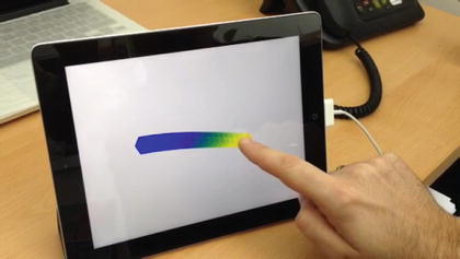
In the field of computational surgery it is frequent to ask for real-time responses. What we exactly mean by the term “real-time” strongly depends on the context but, in essence, it means that we are asking a computer for a response that ranges between 1 kHz for surgery training systems equipped with haptic peripherals to some seconds or minutes in surgery planning applications. But in this last example simulations tend to include long-term behavior of the surgery outcome.
These requirements are extremely astringent if one takes into account the difficulty associated with surgery: highly non-linear soft living tissues, distributed contact, fluid–solid interaction, multi-scale phenomena (that go from the centimeter scale to the sub-cellular scale of gene regulatory systems [2]). Therefore, many computational strategies have tried to pre-compute off-line as many things as possible, and to store them in memory for fast and easy-to-access posterior usage, just like traditional vademecums did. For instance, the so-called fast finite elements for surgery simulation [4] employed static condensation of finite element matrices for linear elastic materials intensively. These matrices could be stored in memory and used when necessary. In essence, when computing  , matrix K −1 could be stored for the sake of speedup.
, matrix K −1 could be stored for the sake of speedup.This can be seen as a sort of very simple computational vademecum, in the sense that K −1 is pre-computed and consulted as often as necessary. However, when dealing with truly non-linear soft living tissues this naive approach is no longer possible, since a consistent tangent stiffness matrix updating should be performed, and this is a very CPU-consuming task. The beam bending vademecum of Fig. 1 could be updated if we consider the computational solution of a non-linear, hyperelastic beam bending problem in which the displacement field u is computed by taking the position of the applied load as a parameter, see Fig. 2, thus by
 where s is the position of the acting load along the boundary of the beam.
This is, roughly speaking, the approach followed in our latest works to develop a means to deal with highly non-linear problems (hyperelastic soft tissues, contact, cutting, etc.) appearing in computational surgery: to make an intensive use of computational vademecums as far as possible. In the subsequent sections we review the main theoretical aspects of this technique as well as some details of its implementation. Other approaches, such as the employ of explicit finite elements, [11, 12], are also equally possible and have given excellent results in recent years.
2 A Vademecum for a Hyperelastic Solid Under Arbitrary Loads
The main drawback of the appealing method sketched in the previous section is that the complexity of the problem (say, the number of degrees of freedom once the problem is approximated by the finite element method, for instance) grows exponentially with the number of parameters of the model, considered as extra-coordinates. To avoid this burden, we have employed a model order reduction technique coined as proper generalized decomposition (PGD). In essence, PGD techniques avoid this exponential growth in the number of degrees of freedom by assuming the solution as a finite sum of separable functions, i.e.,
 In this approach there are two main aspects to be discussed: how to determine the functions F i and G i and how to determine how many of these functions are necessary (i.e., the precise value of N).
Determining functions F i and G i is made by a greedy algorithm [5] that gives rise to a non-linear problem for each sum (even if the original one is linear), whose solution can be obtained by your favorite linearization technique. We have made an intensive use of fixed-point, alternating directions algorithms to this end, with very satisfactory results [13, 14]. The number of terms, N, in turn, can be determined by an appropriate error estimator [1].
As usual in the FE method, PGD considers the weak form of the equilibrium equations (balance of linear momentum) without inertia terms. The (doubly-) weak form of the problem, extended to the whole geometry of the organ, Ω, and the portion of its boundary which is accessible to load during surgery,  , consists in finding the displacement
  such that for all
  :
:
where  represents the boundary of the organ, divided into essential and natural regions, and where
  , i.e., regions of homogeneous and non-homogeneous, respectively, natural boundary conditions. Here,
  , where δ represents the Dirac-delta function and e k the unit vector along the z-coordinate axis (we consider here, as mentioned before, and for the ease of exposition, a unit load directed towards the negative z axis of reference).
, consists in finding the displacement such that for all :(1)
represents the boundary of the organ, divided into essential and natural regions, and where , i.e., regions of homogeneous and non-homogeneous, respectively, natural boundary conditions. Here, , where δ represents the Dirac-delta function and e k the unit vector along the z-coordinate axis (we consider here, as mentioned before, and for the ease of exposition, a unit load directed towards the negative z axis of reference).The Dirac-delta term is then regularized, and approximated by a truncated series of separable functions in the spirit of the PGD method, i.e.,
 where m represents the order of truncation and
  represent the jth component of vectorial functions in space and boundary position, respectively.
represent the jth component of vectorial functions in space and boundary position, respectively.The key aspect of the method here proposed is that PGD techniques efficiently construct the computational vademecum u(x, s) by constructing, in an iterative way, an approximation to the solution in the form of a finite sum of separable functions [6]. If we assume that the method has converged to a solution, at iteration n of this procedure,
where the term u j refers to the jth component of the displacement vector, j = 1, 2, 3, and functions X k (x) and Y k (s) represent the separated functions used to approximate the unknown field, obtained in previous iterations of the PGD algorithm. At this stage, the objective of PGD is to provide the solution with an improvement given by the (n + 1)th term of the approximation,
where R(x) and S(s) are the sought functions that improve the approximation. In an equivalent manner, admissible variations of this displacement field will be given by
(2)
(3)
Of course, the price to pay during this procedure is that, even if the original problem is linear, PGD needs for the solution of a non-linear problem, i.e., to determine a product of functions, see Eq. (3). We describe now a practical way to do this, although the reader can think of any linearization method available in the literature.
For the computation of S(s) assuming R(x) is known, following standard assumptions of variational calculus, we have