Fitting Models to Data

(1)

Department of Mathematics, University of Florida, Gainesville, FL, USA

6.1 Introduction

In the previous chapters, we have learned to develop both simple and complex epidemic models and to perform some partial analysis on them, such as computing the reproduction number. It has become clear that multiple models can be developed to describe a particular epidemic. Which models are good, which are bad, and how can we discriminate among them? Much of the answer to this question is in the realm of statistics, but we will introduce some basic techniques here to address such a question.

After composing a model, perhaps one of the most important steps is to compare the model with data or perform what is often referred to as validation. Model validation is the process of determining the degree to which a mathematical model is an accurate representation of the real-world data [133]. An excellent introduction to model validation can be found in [68]. In mathematics, validation is often not used with the majority of models analyzed, which are never connected to data. Linking our models to data is necessary, for it helps us not only to gain more confidence in the model that we have created, but also to obtain realistic estimates of the parameters.

In Chap. 2, we used data on influenza in an English boarding school to estimate the parameters, so the number of cases predicted by an SIR model compared well with the data. This example is a good illustration of how models can be connected to data, but the approach taken relies heavily on the fact that an implicit solution to the SIR model can be obtained. In Chap. 3, we fitted a number of single-equation demographic models to the world population data, but we again used the fact that the solutions to these models could be explicitly obtained. This is not the case with most models that we create or encounter. In this chapter, we approach the problem from a general perspective.

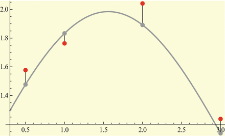
We assume that we have data in the form of a time series for one or more of the classes in the model. Data could be given on the prevalence of the disease, as was the example with influenza in the English boarding school; it may be given on the incidence; and sometimes, it may be given on the number of recovered individuals. We recall that curve-fitting or calibration is the process of identifying the parameters of the model so that the solution best fits the data. What does it mean for a solution to best fit the data? Clearly, ideally, we would like the solution to pass through all the data points. This type of fit is called interpolation. However, interpolation is not always the best approach to fit real data, since the data may contain errors, and capturing every tiny change in them may be impractical. A better way to fit the solution to the data is the least-squares approach. In the least-squares approach, we assume that the time coordinates of the data are exact, but their y-coordinates may be noisy or distorted. We fit the solution curve through the data (see Fig. 6.1) so that the sum of the squares of the vertical distances from the data points to the point on the curve is as small as possible. In particular, suppose we are fitting the prevalence I(t), and we are given the data $\{(t_{1},Y _{1}),\ldots,(t_{n},Y _{n})\}$ . Then we consider the sum-of-squares error:

$\displaystyle{\mathrm{SSE} =\sum _{ j=1}^{n}(Y _{ j} - I(t_{j}))^{2}.}$

The sum-of-squares error SSE is a function of the parameters of the model. So the basic problem is to identify the parameters such that the SSE is as small as possible:

$\displaystyle{\mathrm{SSE}\longrightarrow \min.}$

Fig. 6.1

Least-squares residuals. The red points are the given data points

Minimizing the SSE is an optimization problem with its own difficulties. Differential equation epidemic models are typically nonlinear and cannot be solved explicitly. Hence, the resulting minimization problem is also highly nonlinear. As a result, in the general case, this problem is solved numerically with the use of computer algebra systems such as Mathematica, Matlab, and R. The code requires two basic components: a differential equation solver and a minimization routine. The minimization is typically performed iteratively. The user specifies initial parameter values, and the computer solves the differential equations with those parameter values, evaluates the SSE, and improves the parameter values so that the SSE is reduced. This process is repeated a number of times until the SSE no longer becomes smaller. One important difficulty is that the minimization process is local, so depending on the initially specified parameter values, a minimum may occur for different sets of parameter values, and the minimal value of the SSE may be different. In practice, it may be advisable to check several sets of initial parameter values and use the smallest SSE obtained.

6.2 Fitting Epidemic Models to Data: Examples

In this section, we will consider a number of examples of fitting ODE epidemic models to data. Of course, one interesting question is, where do the data come from? There are several ways of acquiring epidemic data. First, a mathematician can work with biologists or epidemiologists who can collect the data. This is typically possible for limited datasets in limited locations. Comprehensive long-term datasets are usually collected by various health organizations such as the World Health Organization (WHO), Centers for Disease Control and Prevention (CDC), and various foundations. Because these datasets are often collected with taxpayer money, they are public and can be obtained by requesting them from the health organization or perhaps obtained online. For instance, if you go to the WHO Data and Statistics website http://www.who.int/research/en/, there are a number of important diseases listed with data and statistics about them. Suppose we are interested in the cholera epidemic that occurred in Haiti after the devastating earthquake of January 2010. The central WHO website gives only the number of yearly cases by country. If we need more resolution, if, for instance, we need monthly or weekly cases, we can google “cholera data monthly.” We may find the data on the Pan American Health Organization website http://new.paho.org/hq/images/Atlas_IHR/CholeraHispaniola/atlas.html. The third possible approach is to obtain the data from published articles. Data in articles are often published as plots. Hence, if we want the actual coordinates, we need to extract them from the plots. There are many routines that can be used to extract values for the points in a plot. One is PlotDigitizer http://plotdigitizer.sourceforge.net. Matlab also has capabilities to extract data values from a plot. To use Matlab, download Matlab’s grabit.zip from the web and unzip it to obtain the Matlab file grabit.m. Then follow the instructions at http://extractdata.blogspot.com/ on how to use it. This is the way we obtained the data on influenza in the English boarding school.

6.2.1 Using Matlab to Fit Data for the English Boarding School

As described in Chap. 2, in January–February 1978, an epidemic of influenza occurred in a boarding school in the north of England. The boarding school housed a total of 763 boys, who were at risk during the epidemic. On January 22, three boys were sick. The table below gives the number of boys ill on the nth day after January 22 (n = 1).

To fit with Matlab, we do not need to know the final size of the epidemic. Once we have the data (Table 6.1), the first question that we have to answer is, what model we should

Table 6.1

Daily number influenza infected boys

Day	No. infected^a	Day	No. infected
3	25	9	192
4	75	10	126
5	227	11	71
6	296	12	28
7	258	13	11
8	236	14	7

^a Data taken from “Influenza in a Boarding School,” British Medical Journal, 4 March 1978

fit to the data? Since these are outbreak data, we need an epidemic model without demography. As we discussed in Chap. 2, the SIR model without demography is appropriate for this case. We recall the model:

$\displaystyle{ \begin{array}{l} S'(t) = -\beta S(t)I(t), \\ I'(t) =\beta S(t)I(t) -\alpha I(t),\end{array} }$

(6.1)

where we have omitted the recovered class.

The next question that we need to address is which model parameters we should fit and which we should pre-estimate and fix. Potentially, we can fit α, β, and the initial conditions—four parameters altogether. We can pre-estimate α from the duration of infectiousness, and the two initial conditions from the given data. For instance, we know from the data that I(3) = 25, and therefore S(3) = 738. The duration of infectiousness is 2–4 days, so we may take α = 0. 3. Even if we plan to fit all these parameters, pre-estimating what we can is useful with the initial guess of the parameters. In addition, to derive the initial guesses for the remaining parameters before using Matlab to fit, we may use Mathematica’s Manipulate command. In Mathematica, we can fix S(3), I(3), and α to the above values and “manipulate” β to obtain a good agreement with the data. Say we set the value β = 0. 0025. With these initial values, we may use Matlab to fit. Below is the Matlab code used for the fitting.

1 function BSFluFittingv1

2 % This function fits the first set of BSfludata to and SIR model

5 clear all

6 close all

7 clc

9 load BSfludat.txt % loading data

11 format long % specifying higher precision

13 tdata = BSfludat(:,1); % define array with t−coordinates of the data

15 qdata = BSfludat(:,2); % define array with y−coordinates of the data

17 tforward = 3:0.01:14; % t mesh for the solution of the differential equation

19 tmeasure = [1:100:1101]’; % selects the points in the solution

20 % corresponding to the t values of tdata

23 a = 0.3;

24 b = 0.0025; % initial values of parameters to be fitted

31 function dy = model_1(t,y,k) % DE

34 a = k(1); % Assignes the parameters in the DE the current

35 % value of the parameters

36 b = k(2);

39 dy = zeros(2,1); % assigns zeros to dy

41 dy(1) = − b * y(1) * y(2); % RHS of first equation

42 dy(2) = b * y(1) * y(2) − a * y(2); % RHS of second equation

45 end

47 function error_in_data = moder(k) % computing the error in the data

54 [T Y] = ode23s(@(t,y)(model_1(t,y,k)),tforward,[738.0 25.0]);

56 % solves the DE; output is written in T and Y

59 q = Y(tmeasure(:),2); % assignts the y−coordinates of the solution at

60 % at the t−coordinates of tdata

64 error_in_data = sum((q − qdata).̂2) %computes SSE

66 end

70 k = [a b]; % main routine; assigns initial values of parameters

73 [T Y] = ode23s(@(t,y)(model_1(t,y,k)),tforward,[738.0 25.0]);

75 % solves the DE with the initial values of the parameters

77 yint = Y(tmeasure(:),2);

79 % assigns the y−coordinates of the solution at tdata to yint

81 figure(1)

82 subplot(1,2,1);

83 plot(tdata,qdata,’r.’);

84 hold on

85 plot(tdata,yint,’b−’); % plotting of solution and data with initial

86 % guesses for the parameters

87 xlabel(’time in days’);

88 ylabel(’Number of cases’);

89 axis([3 14 0 350]);

94 [k,fval] = fminsearch(@moder,k); % minimization routine; assigns the new

95 % values of parameters to k and the SSE

96 % to fval

99 disp(k);

100

101 [T Y] = ode23s(@(t,y)(model_1(t,y,k)),tforward,[738.0 25.0]);

102 % solving the DE with the final values of the

103 % parameters

104

105 yint = Y(tmeasure(:),2); % computing the y−coordinates corresponding to the

106 % tdata

107

108 subplot(1,2,2)

109 plot(tdata,qdata,’r.’);

110 hold on

111 plot(tdata,yint,’b−’);

112 xlabel(’time in days’); % plotting final fit

113 ylabel(’Number of cases’);

114 axis([3 14 0 350]);

115

116

117 end

We run the Matlab code above. It tells us that the original SSE is equal to 7. 2 ∗ 10⁴. After the optimization, the newly computed parameters are α = 0. 465 and β = 0. 00237. The new SSE is 4 ∗ 10³. We can run the code, taking as an initial guess the parameters we computed in Chap. 2, and Matlab will improve on those, too. In general, the use of computer algebra systems such as Mathematica and Matlab is the best approach to obtain a good fit of the model solution to the data. The newly computed value of α gives the duration of the infectious period as $1/\alpha = 2.15$ days. This infectious period is meaningful, since infected students showing symptoms were quarantined. We should always ask ourselves whether the computed parameters have a sensible biological interpretation. If that is not the case, we should refit, using upper and lower bounds for the parameters.

Using Mathematica’s NonlinearModelFit command, we fitted the model to the data and obtained the same best-fitted parameters as Matlab. One advantage of Mathematica’s NonlinearModelFit is that it can provide many types of statistics that can help us judge the goodness of the fit. One such statistic is the residuals. The residuals are defined as the differences between the y-coordinates of the data points and the corresponding value of the solution. In particular,

$\displaystyle{\mathrm{residuals} =\{ Y _{j} - I(t_{j})\vert j = 1,\ldots,n\}.}$

The best-fitted solution with Mathematica and the data are plotted in Fig. 6.2(left). The residuals are plotted in Fig. 6.2(right).

Fig. 6.2

The left figure shows the fit of an SIR model with the English boarding school data. The right figure shows the distribution of the residuals of the fit in the left figure. Residuals are randomly distributed. Mathematica plots residuals in time starting from t = 1 rather than starting from t = 3

If the fit is good, the residuals should be randomly distributed. Examining the residuals in Fig. 6.2(right), we can conclude that the fit is reasonably good. Mathematica can also provide 95% confidence intervals. A 95% confidence interval (CI) is an interval calculated from many observations, in principle different from data set to data set, that 95% of the time will include the parameter of interest if the experiment is repeated. The CI for the above fitting are [0. 4257, 0. 5037] for α and [0. 0022099, 0. 00254] for β.

6.2.2 Fitting World HIV/AIDS Prevalence

Human immunodeficiency virus (HIV) infection is a disease of the immune system caused by the HIV virus. HIV is transmitted primarily via unprotected sexual intercourse, contaminated blood transfusions, and from mother to child during pregnancy, delivery, or breastfeeding (vertical transmission). After entering the body, the virus causes acute infection, which often manifests itself with flulike symptoms. The acute infection is followed by a long asymptomatic period. As the illness progresses, it weakens the immune system more and more, making the infected individual much more likely to get other infections, called opportunistic infections, that are atypical for healthy individuals. There is no cure or vaccine against HIV; however, antiretroviral treatment can slow the course of the disease and may lead to a near-normal life expectancy.

Because people with HIV now live longer, even though the incidence of HIV is declining, the number of individuals infected with HIV or having advanced-stage AIDS is still slowly increasing worldwide. The United Nations, in their Millennium Development Goals Report 2010, gives the number of people living with HIV [122] as well as the incidence and the number of deaths from HIV worldwide. We include the prevalence data in Table 6.2.

Table 6.2

Prevalence (in millions) of HIV worldwide 1990–2011. 1990 gives t = 0

Year	Time (in years)	Prevalence	Year	Time (in years)	Prevalence
1990	0	7.3	2001	11	29.0
1991	1	9.2	2002	12	30.0
1992	2	11.3	2003	13	30.8
1993	3	13.5	2004	14	31.4
1994	4	15.9	2005	15	31.9
1995	5	18.3	2006	16	32.4
1996	6	20.6	2007	17	32.8
1997	7	22.7	2008	18	33.4
1998	8	24.6	2009	19	33.3
1999	9	26.3	2010	20	34.0^a
2000	10	27.8	2011	21	34.0^a

^a Other sources

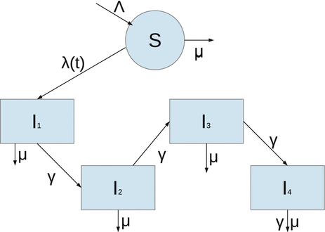
Our main objective is to determine a model that can be fitted to the data. The simplest HIV model is the SI epidemic model with disease-induced mortality. However, this model does not fit the data well. The main reason for that, perhaps, is the fact that a simple SI model has an exponentially distributed time spent in the infectious stage, that is, the probability of surviving in the stage declines exponentially. That is not very realistic for HIV, where the infectious stage is long and the duration is subject to significant variation. That requires that the distribution of the waiting time in the infectious class have a nonzero mode. To incorporate this effect, a typical approach is to use Erlang’s “method of stages.” This approach is primarily applied with stochastic HIV models, but its deterministic variant requires the infectious period to be represented as a series of k stages such that the durations of stay in each stage are independent identically distributed exponential variables [79]. To this end, we divide the infectious class I(t) into four subclasses: I ₁(t), I ₂(t), I ₃(t), I ₄(t) with an exit rate γ. Individuals in all four stages are infectious and can infect susceptible individuals S(t). Denote by I(t) the sum of all infectious classes:

$\displaystyle{I(t) = I_{1}(t) + I_{2}(t) + I_{3}(t) + I_{4}(t).}$

We further assume that the force of infection λ(t) is nonmonotone and is given by

$\displaystyle{\lambda (t) =\beta e^{-\alpha I(t)/N(t)}I(t)/N(t),}$

where N(t) denotes the total population size:

$\displaystyle{N(t) = S(t) + I_{1}(t) + I_{2}(t) + I_{3}(t) + I_{4}(t).}$

This force of infection is sensible for HIV, since as the infection spreads, it is likely that the remaining susceptible individuals become more cautious about their contacts and potential exposure to HIV, and the force of infection begins to decline.

The flowchart of the model is given in Fig. 6.3. The model becomes

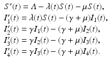
$\displaystyle{ \begin{array}{l} S'(t) =\varLambda -\lambda (t)S(t) -\mu S(t), \\ I_{1}'(t) =\lambda (t)S(t) - (\gamma +\mu )I_{1}(t), \\ I_{2}'(t) =\gamma I_{1}(t) - (\gamma +\mu )I_{2}(t), \\ I_{3}'(t) =\gamma I_{2}(t) - (\gamma +\mu )I_{3}(t), \\ I_{4}'(t) =\gamma I_{3}(t) - (\gamma +\mu )I_{4}(t).\end{array} }$

(6.2)

The last exit rate γ from the class I ₄ is considered to be disease-induced mortality.

Fig. 6.3

Flowchart of the HIV model

To fit the model to the data, we first have to decide in what units to fit. The data are given in millions, and as such, they are neither too large nor too small as numbers. If the numbers we fit are too large or too small, the round-off errors may be large, and the fit may be bad. Therefore, we need to use units that make our numbers reasonable. Furthermore, we will fit in years. After we have decided on the units, we have to decide which parameters to fit, and which to pre-estimate. This decision may have significant impact on the fit. We decide to fix Λ and μ as well as the initial values. The current natural mortality rate of humans can be taken to be 1∕70. Because the current world population size is 7 billion, that is, 7000 million, then if we take that to be the equilibrium population, we have $7000 =\varLambda /\mu$ . We estimate that Λ = 100 million people per year. We further assume that in 1990, all individuals infected with HIV were actually in class I ₁. Hence, S(0) = 6992. 7 and I ₁(0) = 7. 3 million people. We set the remaining initial conditions to zero. In this fitting, we do not fit the initial conditions. We fit α, β, and γ. We fit both with Mathematica and Matlab, but this time, the best-fitted parameters are slightly different. Matlab obtains α = 260. 4972, β = 0. 334547, and γ = 0. 339958755. The SSE = 0. 47 with these parameters. Mathematica’s best-fitted parameters with their standard errors and 95% CI are given in Table 6.3. These results from Mathematica are obtained when the initial values of the parameters are the results from Matlab α = 260, β = 0. 33, and γ = 0. 3399. The standard errors are small, so the parameters are well identified. The fit obtained by Mathematica is shown in Fig. 6.4 together with the residuals. The residuals do not look random, which suggests that a different model might capture the shape of the data better. Nonetheless, the residuals are small, and the fit is reasonably good. We interpret the best-fitted parameters. The only fitted parameter that has biological meaning is γ, where 1∕γ is the time spent in each of the infectious classes. Since γ ≈ 0. 34, it follows that $1/\gamma = 2.94$ . Hence, the time spent in each class is approximately three years, which is reasonable.

Fig. 6.4

Left: the solution with the best-fitted parameters alongside the data for the HIV model. Right: the residuals of the fit in the left figure

Table 6.3

Mathematica’s best-fitted parameters with standard errors and 95% CI

Parameter	Estimate	Standard error	95% Confidence interval
α	253.567	5.84757	[241.282,265.853]
β	0.332276	0.00298656	[0.326002,0.338551]
γ	0.349035	0.00700517	[0.334318,0.363753]

6.3 Summary of Basic Steps

When you prepare to fit a mathematical model to data, think about the following basic steps in the fitting process:

Examine your data. Are the values involved too large or too small? If yes, determine units that allow you to work with average-size numbers.

Choose your model. Is your model sensible for the disease you are modeling? Should your model include demography? Decide whether your data are epidemic or endemic. What is the time span modeled?

Decide which model parameters to fit and which to pre-estimate and fix. Don’t forget that the initial conditions for the differential equations are also in the parameter set. Never fit more parameters than the number of data points.

Only gold members can continue reading. Log In or Register to continue

Stay updated, free articles. Join our Telegram channel

Tags: An Introduction to Mathematical Epidemiology

Nov 20, 2016 | Posted by admin in PUBLIC HEALTH AND EPIDEMIOLOGY | Comments Off

Basicmedical Key

Fastest Basicmedical Insight Engine

Fitting Models to Data

6.1 Introduction

6.2 Fitting Epidemic Models to Data: Examples

6.2.1 Using Matlab to Fit Data for the English Boarding School

6.2.2 Fitting World HIV/AIDS Prevalence

6.3 Summary of Basic Steps

Like this:

Related

Stay updated, free articles. Join our Telegram channel

Full access? Get Clinical Tree

Basicmedical Key

Fastest Basicmedical Insight Engine

Fitting Models to Data

6.1 Introduction

6.2 Fitting Epidemic Models to Data: Examples

6.2.1 Using Matlab to Fit Data for the English Boarding School

6.2.2 Fitting World HIV/AIDS Prevalence

6.3 Summary of Basic Steps

Share this:

Like this:

Related

Related posts:

Stay updated, free articles. Join our Telegram channel

Full access? Get Clinical Tree