Algebraically:

where j is the subscript for the columns (brand), I is the number of rows (in this case, 2), and n is the sample size in each cell (in this case, 5). It’s just the squared differences between the column means and the grand mean (with a sample size diddle factor).
TABLE 9–1 Ratings of satisfaction for different condom brands by circumcised and uncircumcised males
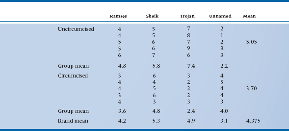
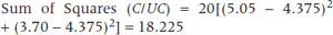
The Sum of Squares (Circumcised/Uncircumcised) is exactly analogous, involving a difference between the two group means and the grand mean, this time multiplying by the number of data in each circumcision group, 20:
And again the algebra looks like:

where now i is the subscript for the rows (circumcision status), and J is the number of columns (4). This is simply the squared difference between the two means and the grand mean (again, with a sample size diddle factor).
The Sum of Squares (Error) is conceptually the same as before, consisting of the difference between individual values and their group mean. This time, though, there are more group means to consider, and so it consists of terms such as:
This turns out to be equal to 24.80.
Once more, with feeling, the equation is:

This is the sum of the squared differences between all the individual data and their respective cell mean (with no diddle factor needed).
However, we have one more term in our bag of tricks—it’s called an interaction.1 As we indicated, it explores the idea that the value of the dependent variable (satisfaction) may relate in some nonadditive way to the value of both factors. Putting it more simply, circumcised males may express a strong preference for some brands and uncircumcised males for other brands.
It is almost easier to see what an interaction is by first considering the appearance of noninteraction. But to illustrate the point, perhaps we can begin with some simpler data. Imagine an experiment similar in design to the present one. A sample of 30 boys and 30 girls is assigned to three different educational programs to teach algebra—lectures, small groups, and computers. There are 10 boys and 10 girls in each group. The goal is to determine what the expected average score in each cell would be if there were no interaction.
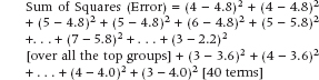
Now, if we knew only that the average score of all subjects was 50%, then our best guess at the expected mean score in each cell is just that, 50%, as we show in Table 9–2 under the first category. But suppose we have a bit more information, namely that girls score, on average, 10% above the mean, and boys, 10% below. We can now add this effect to the information and determine that the best estimate for the cell means in the top row is now 40% and in the bottom row is 60%, as shown in Table 9–2 under the second category.
Now let’s add some more information. Computers beat lecturers by 10%, and lecturers beat small groups by 10%.2 If we add in these effects, we would guess that the expected values in the cells are as shown in Table 9–2 under the third category.
TABLE 9–2 An example of predicting cell means from overall differences
But so far there is still no interaction among factors. The extent to which the actual cell means depart from this picture of expected means is a measure of the interaction between teaching method and gender. So, for example, if boys did much better on computers and worse in groups, whereas girls did better in groups and worse on computers, the Boy-Computer mean would be higher than 50, the Boy-Group mean would be lower than 30, the Girl-Computer mean would be lower than 70, and the Girl-Group mean would be higher than 50. The data might look like that in Table 9–2 under the fourth category. This would constitute an interaction between gender and teaching method. Note that the marginal differences remain the same as in the third category.
The extent to which the actual cell means depart from this picture of expected means is a measure of the interaction between teaching method and gender. The calculation of expected means is also called an additive model.
The interaction between two variables is the extent to which the cell means depart from an expected value based on addition of the marginals.
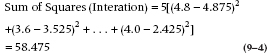
Applying the logic to our present data, on the average, Brand R is a bit below par—4.2 versus 4.375, or 0.175 points. And on the average, uncircumcised men really do have more fun—5.05 versus 4.375, or 0.675 points better.3 So we would predict (if the effects simply added together) that uncircumcised males using Brand R would be up 0.675 from the mean, and down from it 0.175 points; so they would be (0.675 − 0.175), or 0.500 points above the overall average, which is (4.375 + 0.500) = 4.875. As we see, they actually average 4.8, which is pretty close to expectation. But if, for example, uncircumcised males scored Brand R at 5.5 when we expected 4.925, and circumcised males averaged 2.9 when we expected (4.375 + [−0.175 − 0.675]) = 3.525, we can suspect some suggestion of a relationship (or an interaction) between circumcision status and condom brand. Of course, taking the usual nonpartisan, noncommercial view favored by academics who haven’t a ghost of a chance at making any entrepreneurial money, we are not specifically interested in the interaction only with Brand R; we want to show an overall interaction across all brands. So we create an interaction term, which is based on the difference between the observed cell means and that which we would expect based on the marginal means. The first and second terms are based on the expected values we have already calculated, and look like:

As usual, though, these must be multiplied by the cell sample size, in this case, 5. In the end, the sum consists of 8 terms, the last of which is the squared difference between the observed value of the bottom right cell, 4.0, and its expected value (4.375 + (3.1 − 4.375) + (3.7 − 4.375) = 2.425, so it all looks like:
And of course we feel duty-bound by now to furnish the masochists with yet another algebraic equation:

This is, then, the sum of the differences between the individual cell means and what we would have expected if there were no interaction, with one final diddle factor n for good measure.
The next step, as before, is to determine the degrees of freedom. This must be done for each Sum of Squares, and it is a bit more complicated than before. For Brand, it’s the same as before—there are four data points (the sums) so df = 3. For Circumcision Status, there are only two data points, so df = 1. For the Error Sum of Squares, each of the eight groups has five data points, which means that the df for each group is 4, and therefore the Error df is 8 × 4 = 32.
Working out the logic of the df for the interaction term can weary the mind beyond repair. But, the simplest way to figure it out is to multiply the dfs of the main effects that enter into it. The df for Brand are 3, and it is 1 for Circumcision Status, so the interaction term will have 3 × 1 = 3 df. The total df must equal the total number of data points minus 1, or 39. From our discussion we have:

so the arcane logic above must be right.
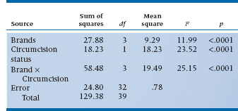
Finally, after all the fooling around, we are ready to put it together into an ANOVA table. Obviously, the table (Table 9–3) has a few more lines in it than did the one-way table.
It is now evident that all the factors are significant. Uncircumcised males do have more fun. There is a difference in brands. Finally, the interaction between the two factors is significant (whatever that means; see below). Note that, although the Sum of Squares and Mean Square for brand are exactly the same as before, the F-test has gone up to 11.99 and the probability has gone down correspondingly. Why? Because we have managed to move some of the variance that was previously contained in the error term into variance attributable to circumcision status and to the interaction between brand and circumcision. As a result, the error term has shrunk. The idea is illustrated in Figure 9–1. Because the Sums of Squares are additive, the sections in the figure have an area proportional to the relevant sum of squares.
Underlying the idea is a fundamental notion, which we mentioned in the beginning of this chapter. Error variance is not really error at all; it is simply variation for which we have no ready explanation. And the more explanatory variables that are introduced—to the extent that they really do explain variance—the smaller will be the unexplained, or error, variance.
It is subject to the law of diminishing returns, however. Because each variable costs at least one df, and usually more, if a variable is not accounting for a significant proportion of the variance, it can result in a less powerful test of the remaining factors. For this reason, some authors state that the term “error” is misleading and replace the term with “within” or “residual.” However, in repeated-measures designs we describe in Chapter 11, we distinguish between “within subject” and “between subject” sources of variance. In deference to terminology, we call the variance term expressing variance not resulting from any of the identified factors in the design, “error.”
TABLE 9–3 ANOVA table for two factors (brand and circumcision)
SUMS OF SQUARES AND MEAN SQUARES FOR FACTORIAL DESIGNS
In the last chapter, we introduced you to the notion of an Expected Mean Square, a sum of variances that together represent the expected value of the calculated mean square. Last time around, it was almost straightforward: the expected mean square between groups was the sum of the variance between groups and the variance within groups, weighted by an n or two here and there; and the expected mean square within groups was the within-group variance.
In the present situation, we have many more possible variances that could enter the sum. As it turns out, the conceptual rule is as follows.
The Expected Mean Square for a main effect or interaction of a variable contains other terms from interactions as well as the error term.
What that bit means is this: the expected mean square for the interaction between Circumcised/ Uncircumcised and Brand contains σ2 (Brand × Circumcised/Uncircumcised) and σ2 (Error). The expected mean square for the main effect of Brands contains σ2 (Brands), σ2 (Brands × Circumcised/ Uncircumcised) and σ2 (Error). All are multiplied by ns here and there, using obscure rules that we will avoid.4
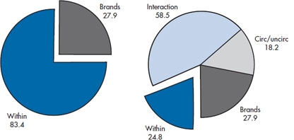
FIGURE 9-1 Sums of squares and interactions caused by factors and interactions.
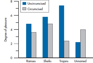
FIGURE 9-2 Pleasure rating by brand and circumcision status.
The effect of all this is that different effects require different error terms. MS(Error) just equals the error variance, σ2(error). The interaction term, MS(Brand × C/UC), contains two terms, σ2(error) and σ2(Brand × C/UC), so the test of the interaction is the ratio of this mean square to MS(Error). The two main effects each contain a variance component for the main effect, σ2(Brand) or σ2(C/UC), as well as the interaction, σ2(Brand × C/UC) and the error term, σ2(error). Strictly speaking, the correct denominator for the F-ratio testing the two main effects should be MS(Brand × C/UC); however, in Table 9–3 we have followed the lead of most computer programs and used MS(Error) as the denominator. The reason for this will be explained shortly, in the section Random and Fixed Factors.
GRAPHING THE DATA (TAKE 1)
In our excitement to explore the delights of factorial ANOVA, we violated one cardinal rule of data analysis—first, graph the data. If we had done so, some of the mysteries of the analysis might have become clear. Look at Figure 9–2.
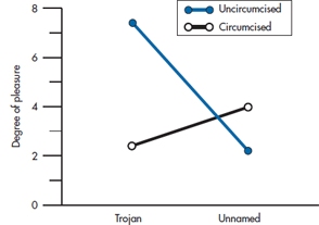
FIGURE 9-3 Interaction between brand and circumcision.
If we just squinted at Brands R and S, all is as expected. Everybody likes S a bit better, and uncircumcised males enjoy sex more. But the mean values of T and U present a very different picture. For some unexplained reason, uncircumcised males express a strong preference for the T brand and circumcised males for the U brand. Therein lies the explanation for the strong interaction term uncovered in the ANOVA. This is magnified in Figure 9–3.
This is only one of several possible types of interactions, some of which are shown in Figure 9–4. In the top left graph, the lines are parallel, but displaced, so the effect of circumcision is the same for both T and U. There are main effects of brand and circumcision status, but no interaction.
In the top right, if we take the average of the two points, one on top of the other, for T and then for U, they are the same, so there is no effect of brand. Similarly, the mean scores for circumcised and uncircumcised are the same, so there is no main effect of circumcision status. But a strong interaction is in evidence because the uncircumcised strongly prefer T and the circumcised prefer U.
Using the same kind of analysis on the lower left, the average for T and U is the same, so there is no effect of brand; but the uncircumcised are always above the circumcised, giving a main effect of circumcised status. Moreover, the lines are not parallel, so there is an interaction. Finally, the bottom right has everything going on—none of the means are the same as any other and the lines are not parallel—so there are both main effects and an interaction.
The extent to which the lines are not parallel is an indication of the presence of an interaction.
If you are still having trouble conceptualizing the idea of interaction, it is synonymous with synergy; the whole is greater than (or less than) the sum of the parts. A match alone has little free energy; a gallon of gasoline alone has little free energy. Put them together, and suddenly you have a lot of energy (and synergy, too).
There is a divergence of opinion about interactions. Some folks hate ’em because if an interaction exists, then they cannot say that the effect of treatment is equal to such-and-such. One version, particularly prevalent in epidemiology, is that one should test only one hypothesis, such as “The drug works”—preferably with only two groups. Obviously the drug companies like this approach because if you are testing their drug against a placebo, there is no chance that some other company’s drug may come out better. This approach has one and only one virtue—simplicity.5 But there are several reasons to contemplate including more than one variable. First, as we showed above, if you can account for some of the variance with another variable—in this case, circumcision status—then you can increase the power of the statistical test of the primary hypothesis.
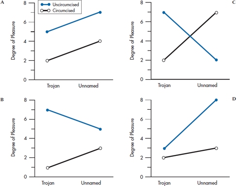
FIGURE 9-4 A, Main effect of brand and circumcision; no interaction. B, Main effect of circumcision; no effect of brand; significant interaction. C, No main effect of brand or circumcision; significant interaction. D, Main effect of brand and circumcision; significant interaction.
Secondly, there is the glory of interactions. In designing our experiments, we actually often go looking for interactions. We believe that it provides much stronger information than a main effect. As an example, one study showed that if you take a group of patients with transient ischemic attacks, aspirin reduces the likelihood of a subsequent stroke by about 20%—but only for men. If the researchers had analyzed the data without including male/female as a factor in the design, they would have concluded that the effect was only about 10%, which in this study would have no longer been statistically significant. In addition, if the effect had been shown to be significant without the analysis by gender, the recommendation would have been to treat everyone with aspirin. The predictable result would have been a few more stomach ulcers and no benefit for the women.
Methodologic benefit is also gained from designing interactions into the study. Suppose we had reason to suspect a bias in the study. For example, perhaps physicians were unblinded and, being skeptical that aspirin could possibly work, put only the patients with a milder stroke episode on aspirin. Now, if all we had was an overall risk reduction of 10%, this bias might indeed explain the results. But if the conclusion is based on an interaction, we must now explain why unblinding of the physicians would result in a bias in assignment to treatment for only the males, which is much less plausible.
As a second example of a deliberately manipulated interaction, it is fair to say that all psychological studies of expertise date back to the studies of a single investigator. Adrian de Groot (1965) studied a group of chess masters, himself included, on a long voyage to America in the 1940s. As it turned out, the single best predictor of expertise in chess was the ability to recall a typical mid-game position. After a few seconds, experts could recall about 90% of the pieces; novices about 20%. Now if he had left it at that and done a t-test on two group means, post-hoc hypotheses would be hanging off every tree. After all, experts are not randomized, so maybe they are self-selected with better memories. Maybe chess playing results in biochemical changes that increase memory. Maybe experts are older, and age, up to a point, results in increased memory performance (this was the 1940s, and most psychologists were studying rat and pigeon memory, not human).
But de Groot didn’t stop there. He also placed the pieces at random on the chess board, and did the same thing. This time there was no effect of expertise—everybody recalled about 20%. So he ended up with an interaction between expertise and real/random position, and the alternate hypotheses came tumbling down. Clearly, expertise in chess resulted in better memory performance in chess. He then went on to theorize that experts are able to “chunk” the data, using memory for previous positions, so as to reduce memory load. The result is that this one paper has directed the last 50 years of research in expertise.
GRAPHING THE DATA (TAKE 2)
We have a confession to make: When we described graphing interactions, we over-simplified things a bit. The problem is that plotting the observed means may give a misleading picture when one or more of the main effects is significant. What we should really do (and we’ll show you how in this section) is to adjust the observed cell means to take these main effects into account. In essence, what we’re doing is going back to the definition of an interaction, that it’s “the extent to which the cell means depart from an expected value based on addition of the marginals,”6 and subtracting the main effects from the cell means. Let’s go back to the example in Table 9–2 and see what difference this makes.
In Part A of Figure 9–5, we’ve graphed the data from the last part of the table, showing the effects of different types of education in algebra for boys and girls. The figure shows us that there is an interaction (as we’ve said), with boys doing best when taught by computer, poorest when taught in a group, and middling when lectured to; for girls, the relationship goes the other way. The graph also tells us that girls do poorer than boys with computers, but better than boys with the other two teaching formats. The problem with trying to interpret the picture in this way is that there are main effects of both gender and teaching method. We remove these effects by subtracting the row and column means from each cell, and then adding in the grand mean. So, for boys taught by computer, the adjusted cell mean is 65 − 40 − 60 + 50 = 15; for boys taught by lecture, it is 40 − 40 − 50 + 50 = 0; and so on. The results are the deviations from the expected value for each cell. If we want to show the results so that the adjusted and unadjusted grand means are the same, we would then add the grand mean (which is 50) to each cell. We’ve done this, and graphed it in Part B of Figure 9–5.
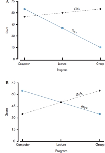
FIGURE 9-5 A, Data from Table 9-2, without adjusting for main effects. B, The same data after adjusting for main effects.
Once we’ve accounted for the fact that girls are better than boys in algebra, and that computers are better than lectures, which in turn are better than group instruction, a different (and more accurate!) interpretation of the interaction emerges: Gender doesn’t make a difference with lecture-based material; boys are better than girls with computerized teaching; and girls are better than boys with group instruction. The moral of the story is clear—don’t try to interpret graphs of interactions or the cell means without first removing the lower-order effects (main effects for two-way interactions; main effects and two-way interactions for three-way interactions; and so on).
If none of the lower-order effects is significant, it’s not necessary to do any adjustment. If only one main effect is significant in a factorial design, you need adjust only for that one, but you don’t lose anything by adjusting for nonsignificant effects.
RANDOM AND FIXED FACTORS
Although it might not have been obvious when we began, there is a subtle difference between our two independent factors. The brand factor contained only a few of the possible “levels” of the factor. If you were to browse the shelves of the local drugstore or other sex shops, you would find dozens or hundreds of other brands. It is almost as if we randomly sampled the brands in the study from a population of possible brands. Nevertheless, our hope is that the results can be applied to other brands. Not exactly of course; if we didn’t study Rainbow Delights, we won’t be able to make a statement about them. But if we don’t find a difference across the four we chose, we presume that we wouldn’t find a significant difference among any four brands. For this reason, brand is considered a random factor.
A random factor contains only a sample of the possible levels of the factor, and the intent is to generalize to all other levels.
The same cannot be said for the circumcised/uncircumcised factor. Either a male is circumcised or he’s not. We need not generalize beyond the two levels of the factor included in the study. For this reason, we call this a fixed factor. A factor can also be fixed if we have other levels of the factor but we do not wish to generalize to them. For example, a study done in the United States might include blacks, whites, and Hispanics. These are only a sample of all possible races, but if the results of the study are applied only to these three, then race remains a fixed factor. It comes down to the statistical notion of population, instead of the street definition.
A fixed factor contains all levels of the factor of interest in the design.
Who cares about the distinction? Unfortunately, you have to when you move to more complex ANOVA designs. As we pointed out earlier, in complex designs the choice of error term becomes a bit complicated, and the choice is further complicated by the fixed versus random issue. In the present example, if brand is a fixed factor, then the denominator for brand is the within-error term; for circumcised/uncircumcised it is the interaction term.
Why is this so? Well, if Brand is a fixed factor, then the interaction between Brand and Circumcision Status is informative, since we can now say something like, “Uncircumcised males prefer Ramses, whereas circumcised males prefer Trojans.” However, if Brand is a random factor, then the four brands we picked are just a sample of all possible brands, and we’re left with a conclusion of the form, “Circumcised males prefer some brands, uncircumcised males prefer other brands.” That really is just error when it comes to deciding which brands are better and which are worse, so the Brand × Circumcision interaction becomes the error term for the test of the main effects.
In the present example, if we treat Brand as fixed, then the correct error term is Mean Square(Error) which equals 0.78, and the F-tests for main effects are as shown in Table 9–3. If, however, we treat Brand as random, then the error term for the main effects is MS(Brand × Circumcision), which equals 19.49, and the F-tests for the two main effects are 0.477 for Brands and 0.935 for Circumcision Status. Neither is significant, of course.
Generally speaking, the effect of treating a variable as random is to reduce the power of the test, which is quite reasonable, since it amounts to adding some component of error derived from the interaction term, and so, in general, the Mean Square(Interaction) will always be larger than Mean Square(Error). Even if the difference between the two mean squares is small (which amounts to a nonsignificant interaction), treating the factor as random may still reduce power, since the degrees of freedom for the interaction is much less (3 instead of 32 in this example), which drives up the value of the critical F-ratio.
Having said all that, without bothering to tell you why it is so, the fact is that most of the time most computer programs never ask.
CROSSED AND NESTED FACTORS
We are not quite through with the generation of jargon yet, all to a worthwhile end, we hope. The design we used to address this question was only one of a number of possibilities. In particular, we ensured that both circumcised and uncircumcised subjects tried out every brand. This was not absolutely necessary because we could have had circumcised men use R and S and uncircumcised men use T and U. If we did, as long as there were equal numbers, we could still have made a perfectly legitimate statement about the differences among brands overall (the main effect of brand) and the effect of circumcision (the main effect of C/UC). However, it would not have been possible to state whether circumcised males preferred some brands and uncircumcised males preferred other brands. In the present design, both circumcised and uncircumcised men sampled all the levels of the brand factor. Thus the two factors are said to be crossed.
Two factors are crossed if each level of one factor occurs at all levels of the other factor.
If we had used the other approach instead, we would have said that C/UC was partially “nested” in brand. A complete nesting would require that we test only two brands, with circumcised males using one, uncircumcised males the other.
Two variables are nested if each variable occurs at only one level of the other variable.
One other variable in the present design is subject, which we chose to make nested; that is, we assigned individual subjects to only one cell or level of both factors. We could have crossed subject with brand (i.e., have each subject try out all brands) but chose not to so we wouldn’t tire out the poor dears.7
Crossing and Nesting are just technical terms, a shorthand way of communicating about experimental designs. But they describe differences that have profound implications for analysis. In general, crossed designs are more powerful because they create the possibility of examining interactions as well as main effects. Conversely, it is impossible or infeasible to cross some factors, and so, of necessity, we end up with nested factors. For example, we cannot have patients both have their appendices out and keep them; similarly, it would be hard to have hospitals doing cost containment one month and not the next.
It’s easy, straightforward, and often very powerful to have crossover drug trials in which a subject gets one drug for a certain period and a second drug for an alternate period. This works nicely because there is a “washout” effect: After some period, the effect of the drug is gone and the subject is okay. Unfortunately, this doesn’t generalize well. Curative drugs such as antibiotics are a one-shot affair. Education interventions hopefully have some lasting effect. And most surgery is a one-way street.
The factor most commonly “crossed” with other factors is the subject or patient. Chapter 11 is devoted to analysis of such designs, which involve using the same patient at various levels of the other factors. Here are some other examples of crossed and nested designs.
- An intervention to convince obstetricians to reduce their rate of cesarean sections was conducted at a random sample of hospitals in the state. Rates of C-sections were determined for each physician in the treatment and control hospital:
Hospital is nested in treatment
Physician is nested in hospital and treatment
- Patients with lupus, 50 males and 50 females, are treated in a randomized trial with cyclosporine. Each patient is randomized to receive either cyclosporine or steroids for 6 weeks. At this point, there is a 2-week washout followed by 6 weeks on the alternative therapy:
Treatment is crossed with gender
Patient is nested in gender, crossed with treatment
- An educational intervention involves completing several computer and paper problems on two organ systems. Three problems are given on each of cardiopulmonary and respiratory systems, represented as both computer and paper questions:
Format (computer/paper) is crossed with system
Problem (e.g., chest pain) is nested within system
Format is crossed with problem
Stay updated, free articles. Join our Telegram channel

Full access? Get Clinical Tree


