• Understand the important contributions of chance, bias, and confounding as potential sources of false epidemiologic associations and apply methods to control for these factors
  
• Describe commonly used measures of morbidity and mortality as they are used in the global setting
  
• Discuss the various types of epidemiologic study designs together with their relative strengths and weaknesses as well as the measures of association they provide
  
• Interpret test results within the context of screening and surveillance with attention to sensitivity, specificity, and predictive value
  
• Apply epidemiologic methods to the control of infectious disease
  
• Distinguish the two types of surveillance and describe the components of a useful surveillance program

Epidemiology is concerned with the identification, measurement, and analysis of factors that may be associated with differences in the health status of populations. The goal of such investigations is to modify these factors to improve the health status of individuals. Classical epidemiology is focused on populations, seeks to identify risk factors, and has been described as the “basic science” of public health. Therefore, some familiarity with epidemiologic methods is essential to the understanding of public and global health. The public health approach can be illustrated by the epidemiologic triad as applied to malaria (Figure 3-1).

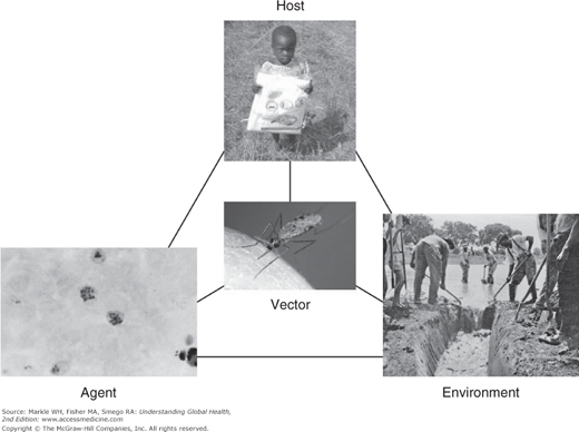
According to this model, disease arises through interactions between a host, environment, and agent. In the case of many infectious diseases, a vector through which the agent is transmitted is also relevant. This model allows opportunities for the interruption of disease transmission to be clarified. For example, in the case of malaria, opportunities might include the use of insecticide-treated bednets for the host, reduced areas of standing water in the environment, destruction of the Anopheles mosquito vector through pesticides, and chemoprophylaxis targeted at the plasmodium.

Note that the public health model takes a very broad view of what constitutes a risk factor for disease. Whereas a traditional biomedical paradigm tends to focus on a small number of causes for a disease, such as a specific microorganism, public health considers more diverse social, economic, and environmental factors as playing a potentially causative role in disease development, each offering an opportunity for intervention.

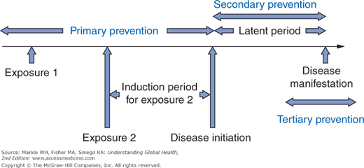
Indeed, there are potentially an infinite number of causative factors, each acting at various points along a timeline as shown in Figure 3-2, which depicts two such factors for simplicity. For each factor, there is an induction period between when that factor acts and when the disease is initiated. After disease initiation, there follows a latent period corresponding to a preclinical phase before the disease is recognized. Preventive strategies can be placed into three groups based on this chronology. The preferred approach is always primary prevention because interventions are made prior to disease initiation, such as vaccination to confer immunity to measles. Screening is by definition a form of secondary prevention as it attempts to identify asymptomatic individuals with disease with the intent of improving treatment outcomes through earlier intervention. Lastly, tertiary prevention does not alter the full manifestation of a disease but seeks to limit the long-term sequelae. Such measures might include physical and occupational therapy following a stroke resulting in hemiplegia.

Although the distinction between epidemiology and biostatistics is not always apparent, biostatistics has a relatively greater emphasis on data gathering and analysis. Accordingly, this field provides a variety of measures used to quantify both disease outcomes (morbidity) and death (mortality). Further, biostatistics offers methods to examine the relationships between variables, especially whether such relationships could have arisen purely as a result of chance, a procedure known as statistical inference.

Chance, Bias, and Confounding

Before reviewing the methods of epidemiology and biostatistics, some understanding of the considerations in determining whether or not associations are valid and causal is needed. An association refers to a relationship in which a change in the frequency of one variable is associated with a change in the frequency of another. For example, x and y may be described as associated if an increase in x also results in an increase in y. Causation is a special type of association in which one condition precedes the other and must be present for the outcome to occur.

Although all causal relationships are forms of associations, the converse is not true; that is, there are many additional reasons that might account for any observed association. To illustrate the difference, epidemiologists classically refer to the example of storks and babies. It can be shown that for many parts of the world, birth rates are higher in those regions with higher populations of storks. However, although these two variables may be positively associated, this is clearly not a causal relationship. The distinction is important because statistics and epidemiology only provide insight into associations. Determining whether an association is causal depends on the application of nonepidemiologic principles. The most widely used are what have now come to be known as the Bradford Hill criteria.1 The most important of these are listed in Table 3-1.

Other than causality, the three most important potential sources for a false association are chance, bias, and confounding. To critically interpret epidemiologic studies, it is essential to address the potential contribution of each of these three factors. If chance, bias, and confounding are not believed to account for an association, the findings are considered valid.

Chance refers to a fluke association. Whenever data are collected in an experiment, unusual results can be obtained in a random manner. For example, a coin may be flipped four times and yield heads on all occasions. Clearly, such unusual associations are more likely to occur when the sample size of an experiment is small. The role of chance is well handled by biostatistics, which provides information on the likelihood that any observed association could have arisen by chance through tests of statistical significance. Generally, a value of 0.05 (5%) is considered a key threshold in determining whether there is or is not an association.

Even when study results are reported as statistically significant, we must still determine whether the association is real. In some studies, a very large number of independent associations are explored. Often, these associations were not specified a priori as hypotheses under study. If 20 such comparisons were made, on average, one will appear to be statistically significant with the use of a 5% or 1-in-20 threshold for significance. Such findings are best described as hypothesis generating because they require further study in which the specific hypothesis is articulated before the data is collected to determine if the association is real.

However, a negative study refers to no association being observed in the study. Two potential explanations must be considered in such a scenario. The first factor is insufficient sample size. A sample size justification should be included in any study that makes explicit the assumptions underlying the methods by which the number of participants was chosen. This sample size calculation depends on the magnitude of the effect under study (smaller effects require larger sample sizes) as well as information about the frequency of exposure and outcome in the study.

When a study is performed, investigators propose the so-called null hypothesis, denoted as H0, which states there is no association between the risk factor and the outcome under study in the population from which the sample has been drawn. After the data are collected and analyzed, the null hypothesis will either be accepted (the findings are not statistically significant) or rejected (the findings are statistically significant). Therefore, four situations can arise, as depicted in Table 3-2. If the null hypothesis is accepted when it is true, a correct decision has been made. If the null hypothesis is accepted when in fact it is false, a type II error, denoted by beta, is committed. Beta is conventionally set at 20% in calculating an appropriate sample size.

Conversely, if one rejects the null hypothesis and concludes that there is a statistically significant relationship between two variables when in fact the null hypothesis is true, one commits a type I error, denoted by alpha. Alpha is set at 5%, again by convention, and corresponds to the threshold to which p values calculated from statistical tests of significance will be compared. If the calculated p value is less than alpha, the null hypothesis is rejected. Finally, if the null hypothesis is rejected when it is in fact false, a correct decision has been made.

Note that type I and type II errors are trade-offs because these are opposite actions. Therefore, a decrease in the likelihood of one increases the likelihood of the other. Because it is generally felt that errors involving incorrect rejection of the null hypothesis are worse, alpha is set at a lower level than that of beta. In planning a study, investigators want to be confident that they enroll a sufficient number of subjects so that if there truly is an association, it can be detected. As can be seen from Table 3-2, this refers to the statistical power of the study and is calculated as 1–beta.

What do these values of alpha and beta really mean? They provide distributions reflective of the values of statistical tests if there is no relationship between the two variables, that is, under the null hypothesis. The process of statistical inference involves the calculation of parameters such as z, t, or chi-square statistics, which all involve a difference between the observed results and those expected under the null hypothesis. As observed results become more extreme from those predicted under the null hypothesis, the likelihood of achieving statistical significance increases. Lower p values correspond to test statistics that fall near one end of this distribution and therefore to findings that are unlikely to have arisen by chance. It should always be borne in mind that the choice of a p value less than 0.05 as justification for statistical significance is both totally arbitrary and historic, with origins in publications dating back to the early 1900s.

Confounding occurs when there is a third variable that is independently linked to both the risk factor and the disease outcome under study. For example, epidemiologic studies published a number of years ago reported an association between consumption of coffee and the development of certain types of cancer. However, it was subsequently shown that the findings were confounded by failure to control for cigarette smoking. Those individuals who drink coffee are also more likely to smoke, and smoking is an independent risk factor for cancer. Although the investigators thought they were comparing groups who differed in the amount of coffee consumed, in reality, they were comparing groups with differing numbers of cigarettes consumed, and it was this latter risk factor that resulted in the observed difference in cancer between the groups.

Confounding can be handled using a variety of approaches, listed in Table 3-3. However, it is obvious that to control a confounder, one must be aware of it. The only method available to control for unknown confounders is randomization in a clinical trial. With appropriate randomization, groups will be the same with respect to every variable, including both known and unknown confounders, and differ only with respect to the intervention under study.

Finally, bias is a systematic error that affects one group preferentially in comparison with another. For example, recall bias refers to the observation that sick people tend to recall more of any exposures, even those that have nothing to do with disease. Many types of bias exist; some of the more common forms are listed in Table 3-4. Because bias is difficult to quantify or measure, it is not easily handled using statistical methods. Therefore, efforts are targeted at minimizing bias in study design through assessment tools that are objective and standardized. A clinical trial offers one of the most powerful methods to reduce bias through blinding. As the name suggests, with this technique a person (the study subject or investigator) is unaware of the intervention (if any) being allocated.

If chance, bias, and confounding are not believed to account for an association, the findings are considered valid. However, many other factors must be considered before one can conclude that valid results are causal and relevant. These factors are discussed in the section on study design later in this chapter. Valid results may not apply to populations other than those included in the study. This consideration relates to the generalizability of the findings.

To study the causes of disease, it is necessary to begin by examining basic health indicators, which include measures of mortality and morbidity. In spite of the widespread use of such indicators, particularly to compare the health status of different countries, it is important to recognize that health involves much more than is reflected by such statistics. In 1948, the World Health Organization (WHO) defined health as “a state of complete physical, mental, and social well-being and not merely the absence of disease or infirmity.” Although this definition has been criticized as utopian, it does highlight the concept that good health is a much more complex notion than simply not having a disease.

In a general sense, most of the measures of morbidity and mortality consist of a numerator such as the number of cases or deaths divided by a denominator representing the population at risk. To measure the size of the population, most countries perform a periodic census, usually every 10 years. Data on births and deaths are collected on a continuous basis and, together with marital status, are collectively referred to as vital statistics.

From a practical perspective, it is usually more difficult to obtain reliable data for the population at risk (denominator for the measures) relative to the number of cases or deaths (numerator). For example, according to the United Nations Statistics Division, the last census completed in the nation of Somalia was in 1987. This lack of information represents a major limitation in understanding the health status of such countries.

The WHO provides basic health indicators together with additional health statistics for all member states in the World Health Report, produced annually since 1995 and available in several languages online at .

Measures of Morbidity

The two key measures of disease frequency are prevalence and incidence. Whereas prevalence refers to the number of existing cases at any one time, incidence is restricted to the number of new cases occurring over a defined period of time.

The two types of prevalence are point and period prevalence. The point prevalence is calculated as the number of existing cases divided by the population at risk at that same time. However, obtaining such instantaneous information is commonly quite difficult, especially for larger populations. In practice, it might require a prolonged period of time simply to assess the population for the number of cases. Suppose a survey was carried out in 2012 in a province of Indonesia to ascertain the number of cases of tuberculosis. The number of cases, divided usually by the mid-2012 population of the province, is a period prevalence. Note that for either type of prevalence, there are no units of time. Therefore, prevalence is not a rate.

The significant limitation in use of the prevalence with respect to understanding trends in disease is that it does not reflect differences in whether a case was recently diagnosed or diagnosed quite some time in the past. For this reason, it is usually preferable to examine the number of new cases by determining the incidence rather than the prevalence.

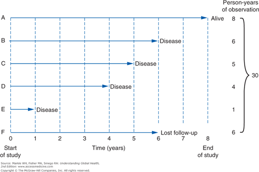
The denominator for incidence is usually expressed as person-years. This is a common metric that allows data from separate observations to be pooled when there is variable follow-up of each individual. For smaller populations, each subject may be considered separately rather than assuming that follow-up is uniform. In such situations, an incidence density is used when there is variable follow-up between subjects. Consider the example shown in Figure 3-3. Only subject A is followed for the entire duration of the study, contributing 8 person-years of disease-free time. However, each of the others can be added, for a total of 30 person-years. The incidence rate or incidence density is then calculated as 4 cases divided by 30 person-years, or 0.13 case per person-year.

There is a clear relationship between incidence and prevalence, namely, prevalence equals incidence times duration, P = I × D. Therefore, factors that increase the duration of disease will increase the prevalence, independent of any change in incidence. The many factors that can influence prevalence and incidence other than changes in the frequency of new cases are shown in Table 3-5.

Measures of Mortality

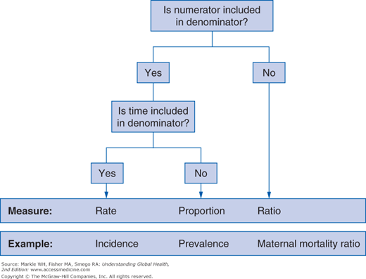
Measures of mortality offer the obvious practical advantage of being based on an objective, easily recognized outcome. Three generic measures—rates, ratios, and proportions—are generally used (Figure 3-4). However, incorrect usage of these terms (especially rate) is very common in the health literature.

The most simple death measure is what is usually referred to as the crude death rate, which, because it contains no unit of time, is not actually a rate. Because the calculated number is usually very small, the figure is conventionally expressed per 1,000 people. For example, the WHO reported that the crude death rate for Botswana was 12.6 deaths per 1,000 persons in 2010. In contrast, the corresponding figure for Brazil was reported to be 6.4 deaths per 1,000 persons.

Obviously, these figures cannot be directly compared because many other differences between these two countries may independently influence mortality. Perhaps most important, Brazil has an older population than Botswana, a confounder that precludes a meaningful direct comparison of rates. In other words, comparing crude death rates may actually underestimate the true difference in health status of these two populations. A variety of approaches can be used to address this limitation. One is to compare age-specific death rates (such as deaths in those 25 to 30 years of age) or cause-specific death rates (such as deaths from pneumonia).

Another method is standardization, which can be done either directly or indirectly. Both types involve the same calculation but are performed in different directions, as illustrated using hypothetical data in Table 3-6. Note that the crude death rate of town A is lower than that of town B. However, closer inspection of the rate within each age stratum shows that all are higher in town A than B. The explanation for this paradox lies in the differing age structure of the two towns: more people are in the older age groups in town B. With direct standardization, the death rate from town A is multiplied by the number of people in that age stratum in town B. The number that arises is the number of deaths given town A’s death rate for each age stratum but using town B’s overall population structure. This is the directly standardized death rate for town A, using town B as a standard. This figure is calculated as follows:

• (4/1,000) × 400 = 1.6 deaths
  
• (4/1,000) × 300 = 1.2 deaths
  
• (6/1,000) × 1,000 = 6 deaths
  
• (10/1,000) × 2,000 = 20 deaths
  
• (40/1,000) × 2,000 = 80 deaths
  
• (150/1,000) × 400 = 60 deaths

Total of 168.8 deaths per 6,100 = 27.7 deaths per 1,000 persons

This figure is now higher than the rate of 23.8 in town B. The conclusion is that, when corrected for age, the mortality is higher in town A than B. This disappearance or reversal of an observed difference when data are stratified and standardized by different levels of a confounder illustrates a concept epidemiologists refer to as Simpson’s paradox.

An alternative approach is to take the death rates of town B and apply them to the age structure of town A. The deaths for each stratum can then be added to yield the number of “expected” deaths if people in town A were dying at the same frequency as those in town B. The observed number of deaths divided by the expected number of deaths yields the standardized mortality ratio (SMR). In this case, the calculation is as follows:

• (2.5/1,000) × 500 = 1.25
  
• (3.3/1,000) × 2000 = 6.6
  
• (5/1,000) × 2000 = 10
  
• (9/1,000) × 1000 = 9
  
• (35/1,000) × 500 = 17.5
  
• (125/1,000) × 100 = 12.5
  
• Total = 56.9
  
• SMR = 67/56.9 = 1.18

The SMR of 1.18 (sometimes multiplied by 100 and expressed as 118) is an indirectly standardized ratio for town A using town B as a standard. Because this figure is greater than 1 (or 100), it provides the same result as the directly standardized rates: the mortality appears to be greater in town A than B when corrected for the different age structures. In general, indirect standardization is used when study populations are smaller. Moreover, the SMR provides an intuitive comparison within one figure, rather than two contrasting rates.

As noted earlier, because it is difficult to obtain denominator data, the proportional mortality ratio (PMR) is frequently used because it only requires more readily available death data. The PMR is calculated as the number of deaths from a specific cause divided by the total number of deaths in the same population. If there are 4,000 total deaths in a population and 200 of these are as the result of injury, the PMR is 0.05, or 5%. The obvious disadvantage of this measurement is that a decline in one significant cause of death must elevate the PMR of another, which can lead to misleading impressions. For example, a successful campaign to reduce injury rates might increase the PMR for cancer only because many individuals who previously might have died at a young age from injuries might now be living long enough to develop an alternative cause of death.

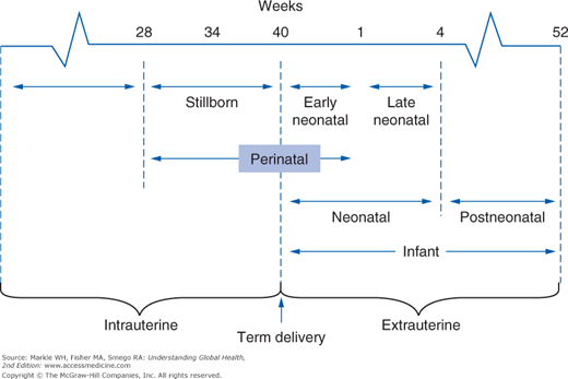
It is also useful to know the case-fatality rate, which is the number of people diagnosed with a disease who die from it. Lastly, a number of reproductive and perinatal fatality rates are commonly used in global health, both because these indicators are quite sensitive to significant disruptions affecting the health status of populations and because deaths in the very young have an enormous public health impact. Figure 3-5 illustrates the eight overlapping fetal and infant periods used to calculate these death rates. Note that for practical reasons, the denominator used is the total number of live births, not the number of pregnancies. Therefore, a woman who dies during the delivery of live-born twins would constitute a maternal mortality ratio of 50%.

Survival Analysis

The concept of case-fatality rate is really only meaningful for shorter periods of observation, that is, for acute diseases. In other situations, it is important to have a more refined measurement that factors in how long each person lived prior to dying. The technique used is referred to as survival analysis, which involves following a group of individuals over a period of time to determine the mortality experience.

In the largest sense, this can be done from birth to death. However, such data would be very difficult to obtain because of the length and effort of follow-up required. As a surrogate, populations at any one time are divided into smaller age groups to create a life table. The WHO provides life tables for all member countries at In this type of survival analysis, the population is divided into the smaller interval of the first year of life because of increased mortality in this group and subsequently is divided into 5-year intervals.

Column ex is the life expectancy at a specified age and the most frequently cited number from a life table. This is clearly a hypothetical number because it is drawn from a cross-section of people all born at different times and assumes that conditions affecting mortality will be stable during a person’s entire lifetime. If ex is taken from the first row of a life table, it represents the overall life expectancy for someone born in that year. If ex is taken from the lower rows of a life table, the number must be added to the age group for that row to calculate the overall life expectancy. For example, the additional life expectancy of a 50-year-old (e50) might be listed as 30.3 years, meaning that the overall life expectancy is 80.3 years (50 + 30.3 years). Note that within each age stratum, there is always an additional period of life expectancy, even in the row for those over 100 years of age. The overall life expectancy is therefore always increasing for each successive age category and is greater than that at birth because those causes of death that might affect younger populations, such as perinatal causes, no longer apply to older populations.

Rather than dividing a large population into arbitrary time intervals and examining how many survived to the beginning of each interval, one can examine a smaller population and determine the exact duration of survival for each member of the group. The procedure is much the same as that used to calculate an incidence density, shown earlier. Instead of birth as used in a life table, the starting point can be the time at diagnosis of a disease or the time when a treatment was administered. Outcomes other than death can also be considered, in which case the term time to event analysis is used. For example, following treatment of breast cancer with mastectomy, time to event analysis may be used with an endpoint of tumor recurrence.

Whenever a group is followed in survival analysis, there will always be those who are lost to follow-up, which might occur either if a subject is lost prior to the end of the study or for those subjects who are still alive at the conclusion of the study. In either instance, we do not know the status of such individuals when they are no longer under observation. In survival analysis, such individuals are referred to as being censored. However, the refinement of survival analysis is that the contribution of survival time prior to censoring is preserved for each subject.

In the example in Table 3-7, 20 subjects are followed for 10 days. On day 4, one subject dies, on day 6 one subject is lost to follow-up, on day 7 there are two more deaths, on day 8 another is lost to follow-up, on day 9 there are three deaths, and on day 10 four more deaths occur. We can generate a Kaplan-Meier curve (Figure 3-6) showing the successive probability of survival for each of these time spans. According to this analysis, an individual’s cumulative probability of survival for this period is 46%. Multiple survival curves can be compared to allow a visual inspection of the different survival experiences.