(1)
Department of Mathematics, University of Florida, Gainesville, FL, USA
10.1 Infectious Diseases in Animal Populations
Infectious disease pathogens affect numerous animal populations. An animal population, by definition, is a collection of individuals of the same species occupying the same habitat. A species is a group of individuals who generally breed among themselves and do not naturally interbreed with members of other groups. Fortunately, familiar baseline models of infectious diseases in humans such as the SI, SIS, SIR, SIRS models also can be used to model diseases in animal populations. There are some very important distinctions, however, that we will discuss below.
Why is it important to study diseases in animal populations?
The simplest and most obvious reason is that a nonhuman species, such as species of fish, birds, and other mammals, represents a much simpler biological system for scientific study than the human species. These species can often be manipulated for better understanding of its properties and dynamics. One such example, in which population dynamics principles were validated through experiments with a beetle population is given in [47].
There is also a practical reason to study animal diseases. Historically, human diseases have been inextricably linked to epidemics in animal populations. Rapid expansion of civilization in the last few millennia has increased the contact at the human–animal interface, through urban and agricultural expansion that encroaches on wildlife habitats, domestication of cattle and other livestock, or simply by keeping pets. Because of such close intimacy between humans and nonhuman animals, viruses and bacteria that cause various animal diseases continuously “jump across the species barrier” and infect humans. Recent examples include HIV, whict came from monkeys; SARS, which came from bats; and avian flu H5N1, which was first found in wild birds. In fact, about 60% of all human infectious diseases have their origin in animal species, and about three-quarters of all emerging infectious diseases of humans—those that are occurring for the first time in humans—have been traced back to nonhuman species. Thus, understanding disease dynamics and ways to control disease in animal populations has tremendous human health implications.
Epidemic models of human populations assume that the population being considered is a closed population, completely separate from the rest of the world. This is rarely true for animal populations. Each animal species is a part of an intricate web of ecological interactions. Interacting populations that share the same habitat form a community. Two fundamental community interactions are competition for resources and predation. Such interspecies interactions impart complex feedback on the dynamics of the diseases in the population that is studied. This necessitates the integration of the principles of infectious disease epidemiology and community ecology.
There are several ways in which the disease dynamics within a population are influenced by the interaction with other species in the community. Here are some of the major ways in which the community interactions influence the host–pathogen dynamics:
Often, a single pathogen simultaneously infects many different species in the community. Even if the pathogen is completely removed from a given host, it may survive in the other hosts and can reinfect the original host. This is of particular concern if one of the species being infected is humans, while another species is an animal species.
Intense competition of the focal host species with the other species in the community can bring down the host population size to threateningly small levels, and a pathogen attack can eventually drive it to extinction.
Predation of the host by other species in the community can regulate pathogen outbreaks in the host species.
Conversely, host–pathogen interactions can feed back and impact the community by weakening the competitive abilities of the affected species.
In this chapter, we will consider the interrelation between infectious diseases and the two principal community interactions: predation and competition. Predation, or predator–prey interactions, refers to the feeding on the individuals of a prey species by the individuals of a predator species for the survival and growth of the predator. Some common examples of predator–prey interactions are big fish eating small fish, birds feeding on insects, and cats eating rats and mice. The predator itself can be of two types—a specialist predator, whose entire feeding choice is restricted to a single prey species, and a generalist predator that feeds on many different prey species. The dynamics of a specialist are strongly coupled to those of the prey, so that any rise or fall of the population size of the prey triggers a consequent rise or fall in the population size of its predator. The interaction between a specialist predator and its prey is modeled by the familiar Lotka–Volterra predator–prey model. By contrast, the dynamics of a generalist predator are only weakly coupled to any particular focal prey species and may not be influenced by the dynamics of the prey. The predation of a focal species by a generalist predator can be modeled by a predator-added mortality on the prey.
10.2 Generalist Predator and SI-Type Disease in Prey
We can begin studying the effect of predation on disease growth in a host population by considering a host to the disease that is also a prey to a generalist predator. We will model the disease dynamics in the prey by the familiar SI epidemic model that we have used for humans. We will also assume that the predator is a “complete generalist,” so that any change of the predator’s population size P is caused by other factors and is independent of the dynamics of the focal prey that we are studying. In mathematical terms, we do not need another equation for the rate of change of P, and P is not a dynamic variable but enters the SI model via the death rate of the prey population as a free parameter. Then we have the following system modeling the dynamics of a host–pathogen interaction with predation:
where Λ is the prey birth rate, β is the transmission parameter, and μ(P) is the prey death rate, which is split into two components:
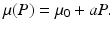
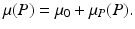 The constant μ 0 is a parameter that lumps death rate from the disease, other natural causes, accidental factors, and so on. The function μ P (P) is the predation-added mortality of the prey that depends on the predator abundance P, taken as a parameter. For simplicity, we assume that μ P increases linearly with P, that is, μ P = aP, where the parameter a denotes the rate at which the predator captures its prey. In general, there should be two different capture rates: a S and a I , for susceptible and infected individuals. For instance, the predator may be able to capture physically weak infected prey more easily than susceptible prey, that is, a I > a S . Here we shall consider two extreme kinds of predation: selective predation, in which the predator attacks only one prey type, leaving the other one alone, and indiscriminate predation, in which the predator attacks all prey types nonpreferentially. For instance, in selective predation of infected prey alone, we have a I > 0, a s = 0, and in indiscriminate predation, we have
  .
.
(10.1)
.10.2.1 Indiscriminate Predation
In this subsection, we assume that the predator preys indiscriminately on all prey types. Hence,
 We obtain the familiar equation
 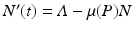 for the total population size of the prey. From this equation, the equilibrium total population size of the prey becomes
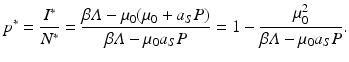
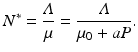 So N ∗ decreases with increasing predator numbers P, as expected. Furthermore, we can solve for the equilibrium number of infected individuals:
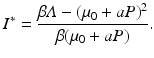
Throughout this chapter, we will call I ∗ the disease load, and the fraction of the infected individuals in the total prey population size will be called the prevalence:
 From the expressions above for the disease load and the total population size, we have that the prevalence is given by
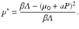
From (10.2) and (10.3), we see that both the disease load and the prevalence are decreasing functions of the predator numbers P. The condition for pathogen establishment requires that the numerators of (10.2) and (10.3) be positive, which gives the familiar threshold condition
 above by Λ∕N ∗ and obtain the inequality
![$$\displaystyle{N^{{\ast}}> N_{\min }^{{\ast}} = \sqrt{\frac{\varLambda } {\beta }}.}$$
” src=”/wp-content/uploads/2016/11/A304573_1_En_10_Chapter_Eque.gif”></DIV></DIV></DIV>Thus, <SPAN class=EmphasisTypeItalic>I</SPAN> <SUP>∗</SUP> = 0 and <SPAN class=EmphasisTypeItalic>p</SPAN> <SUP>∗</SUP> = 0 when <SPAN class=EmphasisTypeItalic>N</SPAN> <SUP>∗</SUP> < <SPAN class=EmphasisTypeItalic>N</SPAN> <SUB>min</SUB> <SUP>∗</SUP>. We have the following interesting result:</DIV><br />
<DIV class=]() While the direct effect of the predator is to harm the prey by increasing its mortality rate, predation can indirectly benefit the prey by keeping its population size low and thereby ruling out epidemic outbreaks.
While the direct effect of the predator is to harm the prey by increasing its mortality rate, predation can indirectly benefit the prey by keeping its population size low and thereby ruling out epidemic outbreaks.
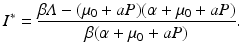
Thus, the pathogen is extinct, I ∗ = 0, when  and equivalently N ∗ ≤ N min ∗. We can obtain the equilibrium prevalence:
![$$\displaystyle{ p^{{\ast}} = \frac{I^{{\ast}}} {N^{{\ast}}} = \frac{(\mu _{0} + aP)[\beta \varLambda -(\mu _{0} + aP)(\alpha +\mu _{0} + aP)]} {\beta \varLambda (\alpha +\mu _{0} + aP)}. }$$](/wp-content/uploads/2016/11/A304573_1_En_10_Chapter_Equ14.gif)
It is clear from this expression that the prevalence p ∗ is not monotone with respect to the predation level P. Looking at the derivative dp ∗∕dP,
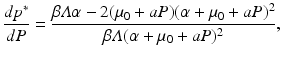 we see that no clear conclusion can be drawn about the sign, and it will depend on the value of the predator population size P. Since for P large enough, the numerator and the whole derivative dp ∗∕dP are negative, if for P = 0 we have
 and the disease load I ∗ decrease with increasing predation pressure P, which tends to give the impression that the epidemic in the prey is weakened in the presence of predation. However, prevalence p ∗, which gives another measure of the disease in the population, increases, at least for low predation level P. The reason is that even though both I ∗ and N ∗ both decrease with increasing P, N ∗ falls faster than I ∗ for low values of P, and therefore the ratio I ∗∕N ∗, which gives the prevalence, increases for those values of P. In other words, while both the population size of the prey and the number of infective hosts are depressed under indiscriminate predation, the proportion of infective individuals in the population increases for low levels of P. The epidemiological significance of this result is that the overall disease burden in the population is reduced, but the risk that a randomly chosen individual is infected can increase with predation, at least at small predation levels.
Get Clinical Tree app for offline access

for the total population size of the prey. From this equation, the equilibrium total population size of the prey becomes(10.2)
(10.3)
above by Λ∕N ∗ and obtain the inequality10.2.2 Selective Predation
In the previous subsection, we assumed indiscriminate predation, whereby the predator’s capture rate a is the same for both susceptible and infected prey. In this subsection, we want to see what happens under selective predation, that is, when the predator attacks either the susceptible prey alone a S > 0, a I = 0, or the infected prey alone, a S = 0, a I > 0. Even though the first scenario is less likely, it can occur in certain situations such as the infected prey hiding in burrows to avoid predation, or the predator may deliberately avoid infected prey to prevent infecting itself. In the case of selective predation of susceptible prey alone, the model (10.1) becomes
The equilibrium disease load is given by
 We see that the equilibrium disease load decreases linearly with increasing predator numbers P. To obtain the equilibrium prey population size, we solve for S ∗ from the second equation above to obtain
 and then use the fact that
  . We obtain
 Hence, the equilibrium prevalence is given by
(10.5)
. We obtainFrom the last expression, we see that p ∗ is also decreasing with increasing P. The threshold predation level for which p ∗ = 0 is
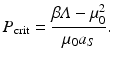 We note that the denominator of p ∗ is positive for all P < P crit.
For the case of selective predation on infected prey alone, the system becomes
Following steps similar to those have taken previously, we get an expression for the prevalence p ∗ as follows:
 We see again that the prevalence is decreasing with increasing P. So the qualitative nature of the result—predation lowers epidemic outbreaks in the prey—is similar to the case of indiscriminate predation discussed in the previous subsection.
(10.6)
In summary, with an SI model, we see that predation reduces disease load and prevalence in the prey population, irrespective of whether the predator selectively attacks either susceptible or infected prey, or indiscriminately preys on both prey types. The main reason is that the incidence rate β S I, which gives the rate at which new infections appear in the host, depends bilinearly on both the susceptible and infected prey. Therefore, whether the predator eats selectively or indiscriminately, it always reduces the incidence β S I, and hence the disease level in the prey population. In the next section, we discuss disease in prey with permanent recovery, and investigate the impact of the predator on the disease load and prevalence of the disease in the prey population.
10.3 Generalist Predator and SIR-Type Disease in Prey
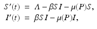
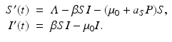
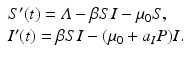
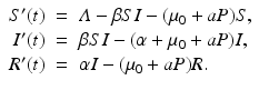
In this section, we consider an SIR model with predation by a generalist predator. The presence of a recovered class of individuals makes a difference. Since the number of recovered individuals R does not directly contribute to the disease transmission, the predation of the recovered prey can have only an indirect effect on disease growth. The addition of a recovered class will give very different conclusions based on the different dietary choices of the predator. We consider the following SIR model with predation of a generalist predator:
The prey death rate μ(P) is defined as before,  . This is the death rate for indiscriminate predation. We will consider two cases of selective predation: predation on infected prey alone,
 ![$$a_{I}> 0,a_{S} = a_{R} = 0$$
” src=”/wp-content/uploads/2016/11/A304573_1_En_10_Chapter_IEq6.gif”></SPAN>, and predation on recovered prey alone, <SPAN id=IEq7 class=InlineEquation><IMG alt=]() 0,a_{S} = a_{I} = 0$$
” src=”/wp-content/uploads/2016/11/A304573_1_En_10_Chapter_IEq7.gif”>.
0,a_{S} = a_{I} = 0$$
” src=”/wp-content/uploads/2016/11/A304573_1_En_10_Chapter_IEq7.gif”>.
(10.7)
. This is the death rate for indiscriminate predation. We will consider two cases of selective predation: predation on infected prey alone, 10.3.1 Selective Predation
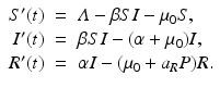
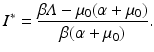
We begin with selective predation on infected prey:
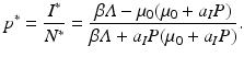
Solving for the disease load in the endemic equilibrium, we have
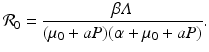
 We compute the basic reproduction number from the requirement that I ∗ > 0,
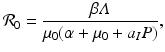
and the condition  . We solve for S ∗ and R ∗ and compute
 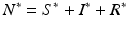 :
:
 The equilibrium prevalence is then given by
![$$\displaystyle{p^{{\ast}} = \frac{I^{{\ast}}} {N^{{\ast}}} = \frac{\mu _{0}[\beta \varLambda -\mu _{0}(\alpha +\mu _{0} + a_{I}P)]} {\beta \varLambda (\alpha +\mu _{0}) +\mu _{0}a_{I}P(\alpha +\mu _{0} + a_{I}P)}.}$$](/wp-content/uploads/2016/11/A304573_1_En_10_Chapter_Equn.gif) It can be seen that p ∗ decreases with increasing predator numbers P at a rate faster than linear. Similar results can be obtained in the case of selective predation on susceptible individuals only, that is,
It can be seen that p ∗ decreases with increasing predator numbers P at a rate faster than linear. Similar results can be obtained in the case of selective predation on susceptible individuals only, that is, ![$$a_{S}> 0,a_{I} = a_{R} = 0$$
” src=”/wp-content/uploads/2016/11/A304573_1_En_10_Chapter_IEq11.gif”></SPAN>. Selective predation on susceptible prey decreases the incidence of the disease <SPAN class=EmphasisTypeItalic>β S I</SPAN> and therefore also decreases the disease load and the prevalence.</DIV><br />
<DIV class=Para>Now we turn to selective predation of the predator on the recovered individuals, that is, <SPAN id=IEq12 class=InlineEquation><IMG alt=]() 0,a_{S} = a_{I} = 0$$
” src=”/wp-content/uploads/2016/11/A304573_1_En_10_Chapter_IEq12.gif”>. The model becomes
0,a_{S} = a_{I} = 0$$
” src=”/wp-content/uploads/2016/11/A304573_1_En_10_Chapter_IEq12.gif”>. The model becomes
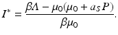
The equilibrium disease load is
 This is an interesting result—the disease load is independent of the predation level P and remains constant with change of P. This happens because both susceptible and infected prey are ignored by the predator, and therefore the incidence rate β S I is unaffected by predation, and so is the disease load I ∗. Furthermore, the condition I ∗ > 0 gives the basic reproduction number
  :
:
which is also independent of the predation level P. An implication of this result is that if the inequality  ,
,
 which then gives equilibrium prevalence:
![$$\displaystyle{p^{{\ast}} = \frac{I^{{\ast}}} {N^{{\ast}}} = \frac{(\mu _{0} + a_{R}P)[\beta \varLambda -\mu _{0}(\alpha +\mu _{0})]} {\beta \varLambda (\alpha +\mu _{0} + a_{R}P) +\alpha a_{R}P(\alpha +\mu _{0})}.}$$](/wp-content/uploads/2016/11/A304573_1_En_10_Chapter_Equq.gif) Unlike I ∗ and
Unlike I ∗ and  , the prevalence p ∗ depends on P, because the equilibrium total prey population size N ∗ depends on P. The behavior of p ∗ with increasing P ∗ is not so obvious, so we consider the derivative of p ∗ with respect to P:
![$$\displaystyle{\frac{dp^{{\ast}}} {dP} = \frac{\alpha a_{R}[\beta \varLambda -\mu _{0}(\alpha +\mu _{0})]^{2}} {[\beta \varLambda (\alpha +\mu _{0} + a_{R}P) +\alpha a_{R}P(\alpha +\mu _{0})]^{2}}.}$$](/wp-content/uploads/2016/11/A304573_1_En_10_Chapter_Equr.gif) This shows that dp ∗∕dP > 0, and therefore, if the prevalence is positive in the absence of predation, i.e.,
This shows that dp ∗∕dP > 0, and therefore, if the prevalence is positive in the absence of predation, i.e., ![$$\mathcal{R}_{0}> 1$$
” src=”/wp-content/uploads/2016/11/A304573_1_En_10_Chapter_IEq17.gif”></SPAN>, it increases continuously with <SPAN class=EmphasisTypeItalic>P</SPAN>. This result is not entirely surprising in light of the fact that the disease load <SPAN class=EmphasisTypeItalic>I</SPAN> <SUP>∗</SUP> remains constant with increasing prevalence. Since we can expect that the total population size <SPAN class=EmphasisTypeItalic>N</SPAN> <SUP>∗</SUP> decreases with increasing <SPAN class=EmphasisTypeItalic>P</SPAN>, we should expect that the ratio, the prevalence <SPAN class=EmphasisTypeItalic>p</SPAN> <SUP>∗</SUP>, is increasing with <SPAN class=EmphasisTypeItalic>P</SPAN>.</DIV><br />
<DIV class=Para>Therefore, once the pathogen is established in the prey, <SPAN id=IEq18 class=InlineEquation><IMG alt=]() 1$$
” src=”/wp-content/uploads/2016/11/A304573_1_En_10_Chapter_IEq18.gif”>, the prevalence decreases with increasing predation level P when the predator selectively attacks susceptible or infected prey only. In contrast, prevalence increases with increasing predation level P when the predator attacks preferentially the recovered prey. This last result, although counterintuitive, can be explained by the fact that by attacking recovered prey alone, the predator decreases total population size without impacting the incidence of the disease β S I.
1$$
” src=”/wp-content/uploads/2016/11/A304573_1_En_10_Chapter_IEq18.gif”>, the prevalence decreases with increasing predation level P when the predator selectively attacks susceptible or infected prey only. In contrast, prevalence increases with increasing predation level P when the predator attacks preferentially the recovered prey. This last result, although counterintuitive, can be explained by the fact that by attacking recovered prey alone, the predator decreases total population size without impacting the incidence of the disease β S I.
(10.8)
(10.9)
. We solve for S ∗ and R ∗ and compute :(10.10)
:(10.11)
,, the prevalence p ∗ depends on P, because the equilibrium total prey population size N ∗ depends on P. The behavior of p ∗ with increasing P ∗ is not so obvious, so we consider the derivative of p ∗ with respect to P:10.3.2 Indiscriminate Predation
As a last case, we consider indiscriminate predation, that is,  . The system in this case becomes
Solving for the equilibrium level of the disease load, we obtain
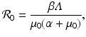
 The condition that the disease load has to be positive, I ∗ > 0, gives the following basic reproduction number of the disease:
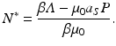
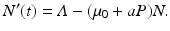
 We see that the reproduction number is decreasing with increasing predation level P. In this case, we can obtain an equation for the total population size. Adding all equations in (10.12), we obtain
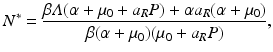
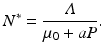
 From the above equation, we obtain the equilibrium total prey population size
We can derive the minimum prey population size N min ∗ needed for persistence of the pathogen by plugging (10.13) into the expression for  and using the condition
 ![$$\mathcal{R}_{0}> 1$$
” src=”/wp-content/uploads/2016/11/A304573_1_En_10_Chapter_IEq21.gif”></SPAN>:<br />
<DIV id=Equv class=Equation><br />
<DIV class=EquationContent><br />
<DIV class=MediaObject><IMG alt=]() N_{\min }^{{\ast}} = \frac{1} {\beta } (\alpha +\mu _{0} + aP).}$$
” src=”/wp-content/uploads/2016/11/A304573_1_En_10_Chapter_Equv.gif”>
N_{\min }^{{\ast}} = \frac{1} {\beta } (\alpha +\mu _{0} + aP).}$$
” src=”/wp-content/uploads/2016/11/A304573_1_En_10_Chapter_Equv.gif”>
. The system in this case becomes(10.12)
(10.13)
and using the condition and equivalently N ∗ ≤ N min ∗. We can obtain the equilibrium prevalence:(10.14)
and the disease load I ∗ decrease with increasing predation pressure P, which tends to give the impression that the epidemic in the prey is weakened in the presence of predation. However, prevalence p ∗, which gives another measure of the disease in the population, increases, at least for low predation level P. The reason is that even though both I ∗ and N ∗ both decrease with increasing P, N ∗ falls faster than I ∗ for low values of P, and therefore the ratio I ∗∕N ∗, which gives the prevalence, increases for those values of P. In other words, while both the population size of the prey and the number of infective hosts are depressed under indiscriminate predation, the proportion of infective individuals in the population increases for low levels of P. The epidemiological significance of this result is that the overall disease burden in the population is reduced, but the risk that a randomly chosen individual is infected can increase with predation, at least at small predation levels.10.4 Specialist Predator and SI Disease in Prey
Specialist predators prey on a given species, which is our focal species. The dynamics of a specialist predator are closely linked to those of the prey. These dynamics are those described by the Lotka–Volterra predator–prey model. In the next subsection, we discuss various types of predator–prey models.
10.4.1 Lotka–Volterra Predator–Prey Models
The Lotka–Volterra predator–prey model was initially proposed by Alfred J. Lotka in the theory of autocatalytic chemical reactions in 1910. In 1925, Lotka used the equations to analyze predator–prey interactions in his book Elements of Physical Biology, deriving the equations that we know today. Vito Volterra, who was interested in statistical analysis of fish catches in the Adriatic, independently investigated the equations in 1926. The equations are based on the observation that the predator–prey dynamics are often oscillatory. The Lotka–Volterra model makes a number of assumptions about the environment and evolution of the predator and prey populations:
The prey population finds ample food at all times.
The food supply of the predator population depends entirely on the prey population.
The rate of change of population is proportional to its size.
During the process, the environment does not change in favor of one species, and genetic adaptation is sufficiently slow.
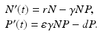
The prey population size N(t) grows exponentially in the absence of the predator and dies only as a result of predation. Thus the prey equation takes the form
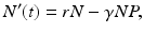 where P(t) is the predator population size, and r is the growth rate of the prey. The rate of predation on the prey is assumed to be proportional to the rate at which the predators and the prey meet, and it is described by a mass action term γ N P. The predator depends entirely for food on the supply of prey and will die exponentially if no prey is available at a natural death rate dm. The equation for the predator takes the form
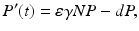 where ε is the conversion efficiency of the predator, that is, ε is a measure of the predator metabolic efficiency by which the biomass of the prey eaten is converted into biomass of the predator. The Lotka–Volterra predator–prey model takes the form